
Guest post by Pat Frank
———————–
“Congress shall make no law … abridging the freedom of speech or of the press…”
On May 24, this year, Jeff hosted my guest-posted Future Perfect analysis here on tAV, which was picked up by WUWT on June 2.
The analysis showed that a cosine+linear fit to the global average surface air temperature anomalies between 1880-2010 pretty much accounted for the entire trend. When the cosine was removed from the anomalies, the residual trend showed no sign of the accelerating climate warming required by AGW.
Wasting no time, Tamino at Open Mind posted three criticisms of my analysis also on June 2, here and here.
Tamino’s criticism consisted of three parts:
1. “there aren’t nearly enough “cycles” to show that global temperature is following a cyclic pattern.”
2. The cosine_linear fit had no physical basis.
3. Arbitrary alternative fits yield a statistically better fit.
I learned about Tamino’s criticisms around June 4, and posted major replies, June 6 and June 12, showing his criticisms were meritless. I also posted replies to other commentators. Tamino properly posted my replies and intercalated his responses into them.
Tamino’s entire analytical response to my June 12 reply consisted of calling me an idiot. He offered no response at all to my reply on June 13.
On June 16 Tamino snipped my reply to a number of posters, writing, “[Response: Enough already.].” And that was the end of that. The reply Tamino snipped is reproduced at tAV here.
The snipped June 13 reply included a link to a Fourier power spectral density (PSD) analysis of the global average air temperature anomaly trend, offered by poster “Bart” at WUWT. Here it is:

This analysis is a frequency analysis that looks for sinusoidal periods within serial data. The strong signal at 0.015 year^-1 says there is a ~65-year cycle within the air temperature anomaly trend.
Bart’s PSD analysis completely and independently corroborated the 60-year cycle found by my cosine+linear fits to the HadCRU and GISS 130-year air temperature anomaly trends.
The snipped response also included a link to a paper by McCabe, et al., 2008, which analyzed an 820-year record of precipitation in Yellowstone, Montana, USA. Their Figure 1 showed the precipitation record and a PSD analysis of it. Here is their Figure:
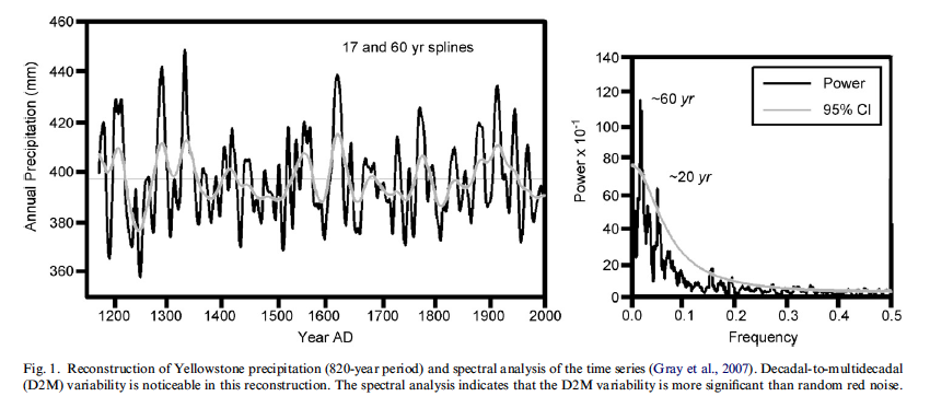
They found 20-year and 60-year cycles in the 820-year precipitation record, which they attributed to long-term variation in SSTs. These periods are identical to the frequencies Bart found in 130 years of HADCRUT3v air temperature anomalies.
Tamino snipped the post showing analyses that perfectly corroborated the cosine fits. The snipped analyses made mush of his entire objection.
Did Tamino snip the post because he couldn’t stand a definitive refutation? We can’t know. However, we can know that, unknowingly or not, Tamino imposed his full censorship at the appearance of an embarrassing contradiction.
The header on my post now comes into relevance. Tamino, of course, doesn’t represent Congress. He is free to censor as he likes on his blog. But I abused no standards. His censorship was whimsical. Censorship contravenes freedom of speech and of the press. It is the instrument of tyranny.
Censorship as Tamino practiced it in this instance violates every spirit of the Constitution, of freedom itself, and of the free rational exchange of ideas. He has implicitly supported this principle: that the open reasoned debate of critical questions can be hamstrung in favor of a sincere prejudice. George III would approve. Tamino’s “Open Mind”: an unintentional irony.

I asked Pat if he would like to put his reply here. Tamino snips everything he doesn’t want people to read and it is important for the MapleLeaf’s of the world to grasp the concepts of the iron fists they unintentionally promote. Censoring an authors defense of his work on a thread critiquing it, is unreasonable yet standard practice at Open Mind.
I think it is within Tamino’s rights to prevent Pat from posting on his site, but it is not within his rights to comment negatively on Pat and then not allow a response.
That’s just chicken sh*t cowardice.
I suggest that Pat submit a complaint to Tamino’s IP server, this is probably a violation of his terms of usage.
The wierd thing about it is that there are multiple (published!) lines of evidence that there is a long term pseudo 65 year oscillation, with proposed physical processes. Certainly Tamino is aware of these published articles. Adding a natural sinusoidal oscillation to a multivariate correlation of historical temperature with GHG forcing history (based on IPCC forcing equations for each compound) turns a crappy correlation into a very good one. With a natural 65 year oscillation in temperatures included, the warming since the late 1800’s is almost perfectly linearly proportional to GHG forcing…. the fit is quite good.
Quite right, Steve. Certainly he’s seen data like this before. (Middle figure.) This is a PSD generated from a roughly 1400-year sequence of proxy data.
This post is a bit dated, but I did a similar look at the HadCrut data a couple years ago, and based on my look at the PDO and AMO cycles nicely fitting a sine wave, I fitted a linear trend against 2 sine waves in the data. Pretty compelling fit, and also a compelling look at what can be expected, on average, in years to come.
http://digitaldiatribes.wordpress.com/2009/02/10/deconstructing-the-hadcrut-data/
Pat has done some great work here as has #5 and many others. I find a two things interesting: first, maybe it’s just me, by why is it that every time someone does a sine-fit and/or a frequency domain transform on temperature data, warmistas and even some luke warmers come out with heavy-duty ad-homs and censorship? Cyclical analysis seems to draw a special sort of bitter, vicious ire. Astrologers. Numerologists. Why?
I mean, wouldn’t it stand to reason that added atmospheric CO2 warming would show up in the temperature signal as some sort of DC offset to a naturally occurring sinusoidal temperature signal? Let me qualify “naturally occurring”. Maybe sunspots or lack thereof. Maybe ocean or deep ocean currents. Maybe cloud formation. Maybe something we haven’t accounted for at all. But at least in geologic time-scales climate is sinusoidal, varying between ice-ages and nice times like right now and in the right-now time frame it is quite obviously sinusoidal as Pat and others have shown. It’s just data. So what?
And in exploring CO2 atmospheric mass fraction (or any other elemental climate contributor), the most obvious first question (to me) is “how does (fill-in-the-blank) pattern-in with the sinusoidal signal? Does said warming goose it on the upside? Minimize it on the downside? Think about what we know about ice-ages and historic mini-ice ages. It isn’t cold winters, but snowy winters and cool summers. Hmmmm….That would be a minimize on the downside kind of event. It isn’t necessarily cold winters, but cool summers and a precipitation pattern that should be focusing our attention in forecasting.
Gosh, it just makes sense to me as a block headed mechanical engineer that we should analyze cyclical patterns as pertains to climate. But anyone that does so is labeled and libeled. And we call this science.
Second thing I find interesting: How can we take serious Mannian hockysticks as opposed to cyclical analysis? That is a rhetorical question. Anything as dynamical as a planetary climate/atmospheric system cannot possibly in any intuitive sense I can even imagine follow a simplistic model as this based upon a single factor. I’m not a climate scientist, but the mechanics of a hockystick based on CO2 just does not stand to reason.
For a self-professed “time series analyst,” Tamino has never struck me as having anything other than a cursory understanding of actual time series analysis tools and interpretation of their results.
Mark
Thanks for hosting my comment, Jeff.
A similar censorious thing happened when I was debating ocean
acidificationde-alkalinization, here. I wasn’t aware of it at the time, but it was Joe Romm’s site. My chief opponent was someone posting as “Dappledwater.” When it was clear the debate was going my way, the moderator (Romm?) snipped my last post, leaving the final word to Dappledwater, and then closed down replies. The site is now dead but the link shows the cached view. Dappledwater continues on, apparently encouraged in his views because he won the debate.Carrick, thanks for your sympathy. 🙂 My sense is that blog censorship is so common that it’s not worth pursuing.
Steve, I don’t understand their repudiation of the published obvious, either. The 1880-2010 calculated temperature change due to GHG forcing (using 1998 Myhre’s equations) is not linear. It’s a concave upwards curve because the rate of GHG production was increasing over most of the 20th century. Only when the rate of increase is a constant, i.e., 1% per year, is the delta T due to forcing linear. A plot of the CRU anomaly fit residual, after removal of the cosine, vs GHG delta-T shows the GHG warming to first curve down through the residual points and then curve up through and emerge above them around the year 2000.
Mark T, whatever else, he’s authored and has a couple of books here and here.
He also has a paper that is somewhat related to the issues at hand.
His criticism of Pat might have left a mark, had it not been for his own selective use of data that tend to substantiate the point that there is a long-period oscillation in climate.
meant to say.. selective ignoring of data…
The last bit is what I was getting at, Carrick. He has clearly studied, and apparently implemented such tools, but doesn’t quite seem to get the interpretation part which implies a lack of a deep understanding of what he is really doing. Inconvenient data doesn’t fit his understanding.
Mark
Yep, he gets really upset when somebody suggests that it may have actually cooled from say 2002-2010, even if that’s what the data suggest…and even if there isn’t any problem for that with respect to AGW (just to his narrative of it).
I have long wondered if a study of temperature data in the frequency domain wouldn’t reveal cyclic periodic excursions that might otherwise be missed. The spectrum plots above are encouraging.
I don’t have the math skill, so this question may be simply exposing my ignorance; can the data be heterodyned to produce a larger effective spectrum to investigate for low and very low frequency cycles? I’d think both first and third order modulation products (sidebands) would be interesting.
cheers,
gary
Have you statistic folks looked at Klyashtorin and Lyubushin’s Cyclic Climate Changes and Fish Productivity? They have performed spectral analyses on various time series, including bristlecone pines, sardines, anchovies, and global temperatures. The dominant periodicities are around 55-60 years.
http://alexeylyubushin.narod.ru/Climate_Changes_and_Fish_Productivity.pdf?
Not sure how scientific or numerologic this is, but look at where the most of the main hot ocean peaks are, at 28 +/_1 year intervals. Would this indicate a periodicity or a harmonic of 55-60 years?
It’s more complicated over land. It depends on the selection of sites. Many sites will give these same maxima, many will give 3, or 2 of them, but others give none at all. Some even go negative in the ‘hot’ years.The pattern over land varies according to which sites are selected into the average calculation of all sites. This rings some bells, because a pervasive forcing like GHG would be expected to be rather universal, would it not?
To me, this gives a strong case to maximise the number of reporting sites, not to minimise. Reason? Just look at the difference between northern and southern hemisphere aggregates, for a possible rationale.
Geoff:
Yes and no. Yes, you can mix (heterodyne) the data to some other region, but no, it will not increase the amount of information present (though you will then be able to extract phase, whatever help that may be.) Mixing does not directly modify the relative contibution of individual components.
Think about it this way: the real (sampled) data has a spectrum that ranges from -f_s/2 to +f_s/2 (f_s being the rate at which the data is sampled.) The negative range is just the complex conjugate of the positive range (except the 0 Hz term.) A mix is nothing more than a barrel shift of the entire spectrum either to the left or right, maintaining all of the original spectrum though the phase of individual terms will change relative to the mixing term. Amplitudes may change a bit depending upon where the terms lie within the bin after mixing, however, but their absolute power does not, e.g., a bin-centered tone that gets shifted to a location between two bins will have half its power in each bin.
Mark
I should add that the example term mixed to a location half-way between two bins will result in an effect known as scalloping as well, but the details are not worth going into from a phone.
Mark
Mark,
Are you familiar with MTM filtering?
Jeff do you mean multitaper method? It assumes you have stable frequency components, I don’t think it does as well as an ordinary Welch periodogram on quasi-periodic time series.
Maybe other people’s experience is different.
Never used it. MATLAB has a function, pmtm, however. Looks interesting, like applying various windows then calculating their FFT cross-correlations.
Mark
Carrick, yes.
I am told that Mann used a form of it in the 90’s. Steve’s been playing around with matching some of his older work. Whatever he used produced a smudged (not so sharp) cutoff frequency compared to a butterworth filter and this is one possibility. Calculate the orthogonal components and delete the hf ones for filtering.
What do you guys think?
It kind of fits the thread because it is billed as better for short time series.
Hmmm… better for analysis purposes, maybe. Not sure about its use as a filter, however.
Mark
Speaking of data filters/smoothers:
http://devoidofnulls.wordpress.com/2011/06/20/low-frequency-variability-in-the-enso-phenomena/
But back to non-amateur statistical analysis:
It seems to me that there is reason to suspect that a pseudo-periodic phenomenon exists in the Earth’s climate/weather system of around sixty years. If this can be identified in one climate variable, examining further and more detailed datasets could help identify mechanistically the origin and nature of this oscillation. Such an analysis would involve, I think, looking at different regions, and at precipitation as well as temperature (especially since this “cycle” was similarly found in a regional precipitation proxy). The “stadium wave” paper of Wyatt et al. is, I think, starting to get at the dynamical/chaotic basis of the phenomenon. Extra detail about the phase alignment could probably be achieved through a complete spatial analysis. Precipitation will hint at some physics.
Ttca:
If you best-fit a sine wave to both PDO and AMO, you get a length of around 60 years on each. Their phases are different, and the lengths are not exact with each other (at least over the data that can be observed) so that when you take a look at a temperature data set that would supposedly incorporate the impact of each of those, you end up with a single overall cycle that appears to be more like 65 years.
The link I provided above takes what appears to be a slightly different approach at the problem, but the results end up being very close to Pat Frank’s. Kind of cool to see, since it’s safe to say I’m not as smart as most other people, and the real advanced statistical stuff thrown around by you guys makes actuaries sound like social kings by comparison 😉
Mann was looking for a way to highlight the thing he was looking for. All well and good when you have a priori knowledge of the thing’s statistics and/or structure, not so good when you do not. Torture data long enough and you can get any confession you desire.
Mark
“Did Tamino snip the post because he couldn’t stand a definitive refutation?”
Yes. Both Tamino and RealClimate pretend to conduct open debate. That goes until they can no longer answer rationally, then you get moderated out. It’s a long know pattern.
Jeff ID:
I meant to reply to this yesterday…we’d have to look at how it compares to other methods for these types of quasiperiodic oscillations.
Just a reminder—a lot of research tools are aimed at problems that involve stationary signals and usually very good signal to noise to boot. (E.g., measuring the acoustic energy generated by a reciprocating engine at constant RPM).
Climate signals from atmospheric-ocean oscillations are neither stationary nor are they substantially above the background fluctuation noise floor.
(OK….gotta work.)
Carrick is correct, though I would note that SNR can be increased by integration, i.e., reducing the noise bandwidth. Of course, knowledge of the noise statistics, as well as the signal statistics is first required. Signals (whatever they may be in such data) that lack stationarity are devilishly difficult to quantize in statistical terms.
Jeff, what exactly is Steve looking at? I may be able to help. Email me.
Mark
Mark, I have a question. What sort of filter would have the following property?
If you take the second difference of the filtered sequence (i.e. difference successively twice), the result is a sinusoidal type of series with varying amplitude and with every second value replaced by zero?
if you can give me a lead on this sort of thing, oplease drop me a comment at my blog site.
Thanks.
Roman,
I think that the MTM method with the with Slepian tapers this zero second derivative could happen by choice of parameters. It is just a guess but when the choices of descriptive frequencies are limited and parameters are hand set, it seems quite possible that every second derivative could be zero.
Jeff, another way of looking at it is that every second term of the original series is the average of the terms on either side. It seems more likely to be a property of the type of smoothing filter itself, rather than only for specific choices of parameters.
Roman, you likely already know this but the Slepian series are constrained to each one having one more crossing over zero than the previous while each being perpendicular to the previous. Filtering of the series occurs after decomposition by the chosen/arbitrary elimination of high frequency signals. It seems quite possible that you might ‘accidentally’ achieve a periodic zero second derivative from such a method. Again, I am spending too much time blogging (or maybe working) to check.
I should add that even checking would be a challenge for me as I am unfamiliar with the method. It just seems possible due to the frequency constraints of the method that it might be every 2, 3 etc. datapoints depending on choice
RomanM,
Are you saying, with input a(n):
step 1. b(n) = a(n) – a(n-1)
step 2. c(n) = b(n) – b(n-1)
?
Mark
Of course, the every other output is zero bit implies more than just a simple filter if the input is arbitrary.
Mark
Oh, I can’t do anything at your blog from my phone… crashes. Damned Droid2 sucks.
Mark
The Yellowstone record got me thinking. I’ve thought of the apparent ~60 year rythm of e.g. AMO (and specifically Barents Sea temperatures) as most likely a coincidental pattern in a rather random process, but now I’m left wondering…
About Tamino: It would be better if we left closed-minded Tamino babbling to himself and his disciples. He blacklisted me after a few posts when I tried to question his silly use of Bayes theorem here: http://tamino.wordpress.com/2010/11/03/how-likely/ (and as you can see, I got a lot of answers I could never respond to).
#36 markT:
I have a smoothed sequence a(n) (along with the original unsmoothed series) for which I am trying to determine the possible types of filtering used.
The second difference I am referring to is d2(n) = [a(n+1) – a(n)] – [a(n}- a(n-1)] = a(n+1) – 2a(n) +a(n-1). The sequence d2(n) has the property that d2(2n) = 0 for all n (i.e all of the even-indexed terms are 0’s) which as I pointed out above, is the same as a(2n) = [a(2n+1) + a(2n-1)] / 2.
There is nothing special about the unfiltered sequence which should produce this result. What types of smoothing filters have this property? I would prefer a reply at my place to discuss this further.
RomanM,
Gotcha, that’s what I thought (work the math on my equations and it is the same result except for the zeroes.) I’ll give you more when I am at my computer. The browser on my phone crashes at your site for whatever reason.
Mark