
Guest post by Tony Brown
——–
Introduction
In March 2009 Leonard Weinstein, ScD provided an interesting thesis entitled ‘Limitations on Anthropogenic Global Warming’ which was carried on The Air Vent and subsequently updated here on this link;
http://docs.google.com/Doc?id=dnc49xz_0fb228shr&hl=en
The author provided much interesting information but in extending the CO2 record back to 1850 naturally used the accepted ice core figures rather than contemporary readings compiled by many leading scientists of the time. These historic CO2 records show a startlingly different view to our current understanding that levels of this trace gas were constant until the 20th century, then escalated rapidly.
Figure 1; The IPCC view of CO2 variations http://climatex.org/articles/climate-change-info/climate-change-impacts-oxfordshire-words-and-pictu/
Consequently in this article I have endeavoured to look at the little known social aspects of CO2 from the 18th Century onwards, in order to demonstrate that accurately measuring this gas was a common place occurrence and that the historic records appear to show that levels have changed little over the past 200 years. As general background, the British Govt then– as now– liked to regulate industries (in this case setting CO2 levels in factories at 900ppm in 1887) and didn’t tend to stipulate legally binding regulations unless they had the means to measure, enforce, and subsequently fine transgressors
Figure 2– Historic CO2 measurements http://www.biomind.de/realCO2/
Inevitably, in trying to tie all the complex elements of the social, regulatory, and scientific story together, there is a great deal of text, links and graphs. For those with limited time to explore the past in detail I have highlighted several ‘KEY’ links which will provide some context to the development of 19th Century CO2 measurements and their subsequent discarding by the IPCC.
The early days
CO2 was not of course discovered by Charles Keeling in 1958 nor even measured by him for the first time around that date. The composition of the atmosphere and the nature of the gases within it had been well understood for many years, partially due to the special circumstances of the mining industry. Interestingly the existence of CO2 and the nature of the atmosphere was recognised as far back as ancient Rome, because of mining; (As an aside many high level Roman mines in the Alps were overwhelmed by ice as the Empire declined as the climate turned down)
Extract from this link;
http://www.cmhrc.co.uk/cms/document/air_flow_2007.pdf
“As recorded by Agricola (1), Pliny (AD 23 to 79) describes how, in Roman times, gases dangerous to humans sometimes occurred in pits and wells. He also describes how they were detected by observing the behaviour of a dog or lighted candle when lowered down the shaft. They were removed by passing a current of fresh air through the workings. In British coal mines one such dangerous gas, almost certainly being encountered by the fourteenth century, was called ‘blackdamp’ or ‘chokedamp’. This was probably in response to the fact that its presence was indicated by naked flames being extinguished and humans suffocating. Blackdamp is now recognised as occurring due to the presence underground of oxidising processes, including breathing humans, burning candles and the spontaneous combustion of coal. Thus it would have been particularly prevalent in workings not scoured by a current of fresh air drawn in from the surface.”
Increasing need for coal in the fourteenth century was undoubtedly spurred by the lurch from the MWP into much cooler times.
The existence of CO2 itself, and its proportions in the atmosphere, was identified as far back as 1756 by Joseph Black, at the start of a rapid increase of chemistry knowledge that laid the foundations for our modern understanding of the subject. The nature of CO2 and its effects were well understood by the late 1700’s and the first measurements of CO2 concentrations were carried out around that time. These became increasingly accurate as the 19th century commenced, with measurements routinely undertaken in various fields including medical, mining and industry.
As far back as March 23 1778 Scheele provided the first definitive reading of the composition of the air and commented on similarity of readings wherever they were made. The following from this document;
http://www.archive.org/stream/carnegieinstitut166carn/carnegieinstitut166carn_djvu.txt
“One figure in this early history of air-analysis shines out above all others that of the scholarly, isolated Scheele. That Scheele may rightly be designated as the pioneer in the study of the chemistry of the air few who examine the literature can deny. His results, while admittedly of no quantitative significance, do nevertheless imply a knowledge of the chemistry of the air, of its composition, and of the possibilities of change in its composition, which was expressed no more clearly by other writers many years later.”
Around this time Cavendish made some 500 samples of air by nitric oxide eudiometer and de Saussure took daily measurements for 3 years, this evolved into the more reliable hydrogen eudiometer. These were very accurate and those scientists taking measurements from around 1800 were well aware of the importance of geography, weather, wind, season, altitude, contamination etc when taking a reading.
CO2 readings from 1790 to 1820 should be considered interesting (and possibly approximately correct) but it is from 1820 onwards that the level of reliability increased enough for us to consider a meaningful proportion of them as a useful record of their time and place. In examining a few of the measurements taken at the time later in this article, it should be borne in mind that they are a fraction of many hundreds of thousands of independent readings taken by many scientists-several of them Nobel winners-from around 1830 to the advent of readings at Mauna Loa in 1957 by Charles Keeling.
It became common place to measure CO2 from the middle part of the 19th century and ensure action if they contravened agreed safety measurements in factories or mines, as laid down in local bye laws-mostly as a ventilation issue. Readings were taken outdoors, indoors or in known hot spots–such as in cotton factories– where allowance was made for spot contamination from sources such as gas lights.
Tyndall-a famous name of course in climate science- worked with Robert Bunsen, who was one of very many who took CO2 measurements.
http://www.tyndall.ac.uk/general/history/john_tyndall_biography.shtml
Tyndall gave lectures to ‘working men’ at mines in the company of Huxley, the author of a compendium of studies of CO2 called ‘Physiography- an introduction to the study of nature” dated 1888. A fascinating section from his biography follows;
“In 1859, aged 39, Tyndall began investigating radiant heat and the acoustic properties of the atmosphere. Part of his experimentation included the construction of the first ratio spectrophotometer which he used to measure the absorptive powers of gases such as water vapour, carbonic acid (Which has the formula H2CO3 and is a name often given to solutions of carbon dioxide in water), ozone and hydrocarbons. Amongst his most important discoveries were the vast differences in the abilities of “…perfectly colourless and invisible gases and vapours…” to absorb and transmit radiant heat. He noted that oxygen, nitrogen and hydrogen are almost transparent to radiant heat, whilst other gases are quite opaque.”
Tyndall’s experiments also showed that molecules of water vapour, carbon dioxide and ozone are the best absorbers of heat radiation and that even in small quantities these gases absorb much more strongly than the atmosphere itself, a phenomenon of great meteorological importance. He concluded that among the constituents of the atmosphere, water vapour is the strongest absorber of radiant heat and is therefore the most important gas controlling the Earth’s surface air temperature. He said that without water vapour the Earth’s surface would be “held fast in the iron grip of frost”. He later speculated how “changes in water vapour and carbon dioxide could be related to climate change.”
By the mid 1850’s it was becoming recognised that in some work places various processes were being carried out that were possibly injurious to the operatives. This effect was commented on by the novelist Mary Gaskell who in 1859 wrote ‘North and South’ where she described the manufacturing processes in the cotton industry. This coincided with a study by Lethbridge in 1862 that looked at the problems of carbon monoxide and dioxide.
The Cotton Cloth factories act of 1889 was subsequently enacted setting actual limits for CO2 at 900 ppm (modern commercial greenhouses operate at up to 1100ppm). Setting a legal limit had been debated in Parliament for some 20 years prior to this and the relative success of the Act subsequently observed in Hansard. (The official record of the UK Parliament)
There was also a variety of legislation enacted to control a variety of problems in mines caused by various gases, including CO2. The various Coal mines acts of 1855, 1887, 1911 refer. The 1887 act identified specific legal limits for CO2. Before the various mine acts could be passed various Royal commissions were set up and some 25 can be accessed from here, commencing in 1842. Concerns often centred round ventilation issues;
http://www.cmhrc.co.uk/site/literature/royalcommissionreports/
In the following book more of the background that led to the Parliamentary Act can be read (page 154 onwards) which makes considerable mention of carbon dioxide in factories and how measurements should be controlled-by-for example- taking into account the gas lighting and the processes used to power various machines. http://216.239.59.104/search?q=cache:yoxDE4U_T94J:www.victorianlondon.org/publications/westlondon-2.htm+cotton+industry+carbonic+acide+levels+victorian+era&hl=en&ct=clnk&cd=7&gl=uk
A complete bibliography of the cotton industry and the activities of the Roscoe commission -who investigated the effects of the carbon dioxide levels for Parliament- can be found here;
http://www.spinningtheweb.org.uk/web/objects/common/webmedia.php?irn=257
Throughout the 19th century the measuring methods had become increasingly accurate, commencing at the start of the century at around plus or minus 3 % until by 1850 accuracy was said to be within 0.1%. Legislation led to a rash of ever more sophisticated methods for measuring CO2, including a patent around 1895. This level of accuracy was perhaps not surprising as the basic principles of chemistry were increasingly well understood as the century had progressed. Further reference to the social elements is here-of particular relevance is the section entitled ‘The first limits’.
http://annhyg.oxfordjournals.org/cgi/content/full/48/4/299
In due course, as more sophisticated machines for measuring CO2 came into general use, market leaders established themselves, including Haldane and Sonden Patterson of Stockholm. Charles Keeling makes references to Prof Haldane who created a highly accurate device for measuring carbon dioxide in the 1890’s which was used in mining and medical situations (exhalation), his obituary linked below confirms his knowledge of the subject.
http://www.dmm.org.uk/archives/a_obit20.htm
The following is in connection with Haldane’s work for the Admiralty in measuring CO2 levels for divers;
http://www.divernet.com/cgi-bin/articles.pl?id=2602&sc=1040&ac=d&an=2602:Grace+under+pressure…
The device he invented became a portable version and was part of the standard equipment in various organisations including hospitals, as can be seen in this inventory;
http://janus.lib.cam.ac.uk/db/node.xsp?id=EAD%2FGBR%2F1919%2FAHRF%208%2F176
This 1912 document has already been referenced in connection with Scheele;
http://www.archive.org/stream/carnegieinstitut166carn/carnegieinstitut166carn_djvu.txt In addition there are two other famous chemistry studies of especial interest, one of which has already been mentioned;
‘Physiography: An Introduction to the Study of Nature’ by T H Huxley published in 1885, where typical values converted to ppm are generally from 327 to 380. The measurements were carried out by Angus Smith and are originally given in his book ‘Air and Rain’ published in 1872. (The 327ppm recording was taken on top of Ben Nevis, Britain’s highest mountain at some 4000 feet). (This latter book is still available for free loan from the UK library service)
So do those early observations of CO2 match other data? There are numerous bibliographies that demonstrate the considerable scientific attention being paid to CO2 at the time and it is apparent that past generations of scientists are much more knowledgeable and meticulous than the IPCC give them credit for; The following information and quotations comes from the 1912 document, except where stated;
As an aside, there was friction even then between the two sides who had their own way of taking samples and who constantly criticised each others science. Kreusler being said to having taken ‘great exception to his critics’ over his methodology to which he retorted they related to ‘but one set of samples which had already been identified as false and withdrawn.’
The following CO2 sample figures (in ppm) are from well observed locations/times and conditions; (some indoors, some countryside)
Nov 1884 036 037 039 041 050 055 0389 0391 040 044 044 048
A week later under the same criteria;
049 540 380 410 416 430 400 370 370 400 440
Feb 1885 sees a set of consistent samples from a rural area;
350 340 340 340 351 and a week later 370 350 360 340 350
In 1902 Krogh took some Greenland samples said to be accurate to .0005 to .01%. measured at 700 ppm
“In a private communication from Dr. Krogh, he reports that a series of experiments made by him in Greenland in 1908 showed oxygen percentages ranging from 20.895 to 20.980, with an average of 20.945. The unusually high carbon-dioxide percentages of former years were not obtained, (up to 700) although two observations gave 0.055 per cent. Dr. Krogh also writes that in 1907 and 1908 Dr. Lindhard of Copenhagen made observations in northeast Greenland (Denmark Haven) using the identical modified Pettersson apparatus described by Dr. Krogh in a former paper. He reports that Lindhard’s results would be liable to about 0.001 per cent error, and they agreed perfectly with those found by himself on the west coast. Lindhard generally found about 0.035 per cent of carbon dioxide, but on one or two days it was below 0.03 per cent, and on 5 days out of 23, 0.04 per cent or more. The maximum value found was 0.062 per cent.”
The very high Greenland figures (620 to 700 ppm) appear absurd and the analysis at the time says;
“The one inexplicable phenomenon is the abnormally high percentage of carbon dioxide found in the air of Greenland by Krogh.” Recent examination demonstrates that there may have been previously unidentified volcanic activity that increased the background figure.
Independent sets of samples from another scientist made in Paris in 1903 registered 300ppm and in 1910 Bay of Genoa Naples; cloudless sky; temp, on Moist 0.034
Equipment evolved quickly throughout the 19th Century; “Eudiometric observations were exclusively relied upon during the first 50 years of the development of air-analysis, but later gravimetric methods were introduced by Brunner and Dumas in which the oxygen was absorbed by copper or phosphorus, and was subsequently weighed. Then there followed a return to the hydrogen-explosion method, which was advanced to the highest degree of accuracy by Bunsen, Regnault, Frankland and Ward, and Morley. Meanwhile the interesting method of Liebig, employing an alkaline solution of pyrogallic acid, and the copper eudiometer of von Jolly made their appearance.”
“Of particular significance is the fact that analyses made on the same samples sometimes showed extremely high values for carbon dioxide, ranging at times from 0.025 to 0.07 per cent.”
(Definition; The art or process of determining the constituents of a gaseous mixture by means of the eudiometer, or for ascertaining the purity of the air or the amount of oxygen in it.)
The document referenced provides hundreds of pages of equipment, techniques, samples readings and tips on ensuring maximum accuracy of readings.
“While the investigation was started primarily to study the oxygen-
content of the outdoor air, it was necessary to determine beforehand the carbon dioxide, since an alkaline absorbent for oxygen was employed; hence practically all the analyses are accompanied by simultaneous determinations of the carbon dioxide in the air. In the especially exact apparatus designed by Sonden and Pettersson, the carbon dioxide is determined to the third or fourth significant figure, but as the amounts of carbon dioxide that were to be used in our apparatus might at times reach 1 per cent, it was impossible to secure this degree of fineness in the calibration of the carbon-dioxide pipette, hence readings can be taken only to one-thousandth of 1 per cent. Consequently, since other methods are better adapted for securing accurate carbon-dioxide determinations, little stress has been laid upon the determinations made in connection with this research, although they are probably accurate to within 0.002 in all cases. The routine outlined was followed with practically no modification from April 5 up to Nov. 3, 1909. “
There then followed a long series of hourly and daily recordings observed in the referenced book, a fraction of which are reproduced here;
Table 50. Results obtained on sample of outdoor air with
first routine, April 5, 1909, 11 h 45 m a. m. 0.029 0.031
Table 51. Analyses of outdoor air made at the Nutrition Laboratory. 1 Series
1909. Apr. 5 onwards almost daily to June 3 and virtually every hour
Then Oct. 18 to December
0.031 .032 .028 .026 .029 .030 .027 .030 .027 .029 .030 .029
.030 .031 .032 .030 .031 .031 .031 .032 .032 .030 .030 .032 .030
.028 .028 ‘.028 .029 .029 .031 .028 .030 .029 .029 .029 .031 .029
.028 .030 .029 .031
Another series Table 52. Results obtained on sample of outdoor air with
second routine, November 4, igog, g b /o m a. m. 0.035 0.036
1909 Pleasant, warm and sunny.
0.034 .033 .034 .031 .029 .028 .029 .031 .032 .033 .032 .030 .030
.031 .031 .031 .032 .034 .032 .029 .031 .032 .030 .030 .028 .033
.031 .031 .030 .028 .028 .028 .028 .029 .030 .028 .031 .031.030
.030 .031 .030 .028 .033 .032 .032 .034 .030 .032 .033 .030 .029
.028 .030 .028 .030 .029 .030 .028 .030 .029 .030 .031 .031 .033
.030 .030 .033 .031 .032 .031 .031 .031
An experiment had to conform to strict criteria;
“…. would be thoroughly mixed and have a fairly constant composition. Employing precisely the same technical routine, samples of the cylinder air were frequently analyzed as a control on the analyses of the outdoor air.” The results of these analyses made between December 3, 1910, and February 9, 1911, are given in table 54.
1911. Dec. 9 2 56 p.m..032
Jan. 21 2 32 p.m. .031
Dec. 10 10 14 a.m. .031 3 43 p.m. .033
Dec. 13 12 02 p.m. .034
Jan. 23 9 37 a.m. .032
Dec. 15 11 52 a.m. .031 10 52 a.m. .033
Dec. 22 2 31 p.m. .033
Jan. 31 10 03 a.m. .032 3 43 p.m. .033
11 30 a.m. .033 4 52 p.m. .034
Feb. 9 .034
At this stage it became pointless to continue recording the information of thousands of samples, as the figures consistently show readings of up to around .034 or so throughout the daily readings made in Dec 1911 through to 1912- the measurement records can all be seen in the document referenced and confirmed in the various bibliographies available;
“The results of analyses of air taken near the laboratory showed no material fluctuation in oxygen percentage during a period extending from April 15, 1911, to January 30, 1912. This constancy was maintained in spite of all possible alteration in weather conditions, changes in barometer, thermometer, humidity, and wind direction and strength; furthermore, the experiments were made before, during, and after the vegetative season. The average result of 212 analyses showed 0.031 per cent of carbon dioxide and 20.938 per cent of oxygen. The analyses of air collected over the ocean, at two different times of the year, and on the top of Pike’s Peak, gave essentially similar results. The average results of all the analyses made in this research of outdoor air are summarized in table 72.”
That CO2 readings became commonplace in Victorian times can be seen here;
“It will be seen, therefore, that since there are a number of simple and accurate methods for determining carbon dioxide, so the time-consuming and complicated determinations of oxygen are entirely unnecessary.”
Comment on Methodology; “The wisdom of taking samples dry is seen from these results, since in all dry samples the percentage of carbon dioxide was found to be always normal.”
These apparently higher than expected historic CO2 figures are noted by this separate study in 1981;
http://www.springerlink.com/content/v4655l63w6342p84/
“Abstract from articles The longest continuous record of measurements of atmospheric CO2 concentration available to date, that was made between 1877 and 1910 at the Montsouris Observatory in the outskirts of Paris, is presented and the methods used and the site are described…..
….Mean decadal values of the Montsouris series show a marked rise in concentration from 283 ppm in the first decade to 313 ppm in the second, with a small and non significant drop to 309 ppm in the third decade of the series. The results of the measurements are thus compatible with the hypothesis that a major and variable non-fossil fuel source of atmospheric CO2 was active during the last quarter of the nineteenth century.”
The link below leads to a 1917 study where the means to analyse CO2 is taken as the norm and viewed as a simple procedure. http://www.jbc.org/cgi/reprint/33/1/47.pdf
That CO2 levels can vary considerably in a year (readings taken weekly and averaged at Mauna Loa) might be surprising, but it does occur;
http://cdiac.ornl.gov/ftp/ndp001a/ndp001a.pdf
The above study by Keeling, (for example a location in Canada) ranges from 360 to 378ppm (seasonal changes amongst others)
The article from the following link examines the concept of urban CO2 domes and contains an interesting diagram;
http://www.co2science.org/subject/u/summaries/phxurbanco2dome.php
Extract; “Idso et al. (1998a) measured air temperature, relative humidity and atmospheric CO2 concentration at a height of two meters above the ground at approximate 1.6-km (1.0-mile) intervals prior to sunrise and in the middle of the afternoon across four transect routes through the metropolitan area of Phoenix, Arizona, during a five-day period in January of 1998. These data revealed the presence of what they called an “urban CO2 dome,” the two-meter-height atmospheric CO2 concentrations of which were found to be as high as 555 ppm at the center of the city.”
The apparent considerable natural variation in CO2-see figure 3-due to ocean to air exchange (amongst other factors) puts the apparently irrational variable figures from the 19th Century onwards into context, yet IPCC AR4 suggests a remarkably constant 285ppm at this time, despite the expected outgasing and inflow caused by variability in ocean temperatures. The IPCC icon is Mauna Loa so it is instructive to go to the oracle so see what that says about variability;-this link shows how observations are made in general;
http://www.mlo.noaa.gov/programs/coop/scripps/co2/co2.html
The following link goes into more detailed specifics;
http://www.esrl.noaa.gov/gmd/ccgg/about/co2_measurements.html#variations
Figure 4 shows the range of the mole fraction in ‘scatter’ measurements whilst figure 5a demonstrates real world conditions and the variation of CO2 in the atmosphere shown in the top part of that graph, and in the bottom section the effect when averaged out over a day, so the 335ppm to 368ppm again puts the observed variability in the historic samples in much better context. The overall effect of taking CO2 measurements at Mauna Loa situated on top of an active volcano at over 3000 m altitude and surrounded by a constantly outgasing warm ocean shall be left to others to debate, but the averaging disguises the considerable daily variability.
Outgasing of CO2 occurs when oceans are warm, interestingly the 1912 readings mentioned earlier contains this note;
“When the air-analyses were resumed in the fall, after a summer of unprecedented heat in Boston…”
“ANALYSES OF AIR FROM PIKE’S PEAK. (14000 feet altitude)
The interesting expedition to the top of Pike’s Peak made by Haldane,
Yandell Henderson, Douglas, and Schneider, in the summer of 1911, was
utilized in that these gentlemen kindly consented to collect samples of air for this research….possibly resulting from the extreme heat of the summer, which had been abnormal for this section.”
There are a number of interim observations we can make before examining in the next section as to why the figure of 280ppm pre industrial became the accepted norm.
* From Victorian times readings were taken widely and frequently
* Measurements were taken by established scientists using reliable methods
* Levels consistently show around 310 and above-with 330/350 frequently attained
* CO2 levels varied considerably throughout the period 1820-1957
* Allowance was made for possible disruptions to readings-for example sources of CO2 were identified-such as from gas lamps
*European CO2 levels immediately prior to the commencement of the Keeling data in 1957 appeared to be around 30ppm higher than he recorded
*Averaging disguises the ranges.
*The current levels of CO2 are not unprecedented if the historic records are accurate
Section Two How 280ppm became the accepted pre industrial norm.
At this stage it becomes necessary to examine why 280ppm became the figure accepted by the IPCC, even though there was overwhelming documentary evidence to show this figure was rather on the low side, and levels were anyway subject to much more fluctuation than modern records seem to indicate. (This paper does not go into the separate subject as to whether temperature rises first, followed by increased CO2, or the timescale of cause and effect)
Anyone reading the following should put themselves into the mindset of those creating the science of CO2 measurements from the 1950’s who were especially influenced by the measurements taken by an amateur meteorologist-G S Callendar- some years previously. The accessibility of data should also be taken into account-we take instant information for granted and can make ready comparison with numerous sources at the touch of a button. In making these caveats we look at this extract from the Book ‘The Callendar effect’ as this gentleman is known as the Father of the AGW theory and is someone who greatly influenced Charles Keeling.
“Callendar’s 1938 paper did not include a citation of Arrhenius’s 1896 paper, although there are many parallels between the two. Callendar analysed just one set of data on atmospheric CO2 content taken at Kew, near London, between 1898 and 1900. These data were taken near a source of CO2 and were analytically very uncertain. From this analysis, he concluded that at around 1900 the free atmosphere over the North Atlantic region contained 274 ± 5 parts per million (p.p.m.) of CO2. Then, after arguing that only a small fraction of the CO2 from combustion of fossil fuels would dissolve in the ocean, he calculated from an estimated global production rate of CO2 the amount that he thought would be there in 1936 (290 p.p.m.), 2000 (314–317), 2100 (346–358) and 2200 (373–396).
With a simple model of the absorption of infrared radiation, he worked out the amount of global warming to be expected from his predicted CO2 levels, concluding that temperature would then have been increasing at a rate of about 0.03 °C per decade. Callendar’s 1938 attribution of early twentieth-century warming to CO2 increase might have been believable if global cooling had not ensued in the 1960s and 1970s.”
Callendar was a noted amateur meteorologist and steam engineer. After reading his papers-and corresponding with him-Keeling used that research as the basis for his own estimates of CO2. From Callendars biography;
“In 1944 climatologist Gordon Manley noted Callendar’s valuable contributions to the study of climatic change. A decade later, Gilbert Plass and Charles Keeling consulted with Callendar as they began their research programs. Just before the beginning of the International Geophysical Year in 1957, Hans Seuss and Roger Revelle referred to the “Callendar effect” — defined as climatic change brought about by anthropogenic increases in the concentration of atmospheric carbon dioxide, primarily through the processes of combustion.”
Callendar examined 19th and 20th century CO2 measurements, and rejected those he considered inaccurate for a variety of reasons, the ones he selected led him to conclude that the pre-industrial CO2 level was about 290 ppm (G. S. Callendar, “The Composition of the Atmosphere through the Ages,” The Meteorological Magazine,vol. 74, No. 878, March 1939, pp. 33-39.) This seemingly low 280/290ppm figure is important, as it is the one that Charles Keeling subsequently accepted.
Among the criteria that Callendar used to reject measurements were any that deviated by 10% or more from the average of the region, and any taken for special purposes such as such as “biological, soil, air, atmospheric pollution”. The first criteria is said to be a rather circular argument, while the second seems to ignore the accuracy of the results. Whatever the validity of these exclusions, it turned out that the mean of 19th century samples he chose to include was 292 ppm. The mean of the samples he had available to include was 335-350 ppm (although these would have been towards the top end of the spread).
Selecting measurements from the low end of the spectrum was robustly justified in the article Fonselius and the history of CO2 measurement carried here;
http://www.someareboojums.org/blog/?p=25
Extract; “Fonselius et al. go on to discuss how CO2 measurements might be improved and collection extended, remarking that in the diagram,(contained in the link) the values used by Callendar and our mean values are encircled and we can see that our values fit in quite well.
This analysis seems at variance with the information now available and that Keeling later came to believe in the accuracy of the old measurements he had previously rejected as being too high is demonstrated in his own autobiography. Ironically Callendar in the last years of his life also doubted his own AGW hypothsesis. Similarly whilst Arrhenius’ first paper on the likely effect of doubling CO2– with temperature rises up to 5C– is often quoted, his second paper ten years later– when he basically admitted he had got his initial calculations wrong-is rarely heard. In this latter paper he estimated a figure of 0.7C for doubling, although the base CO2 measurement used might be contentious.
During the 19th century –and up to 1957 with the inception of the monitoring station at Mauna Loa– it was widely accepted that the ‘normal’ level for Co2 was 400ppm. As already mentioned the catalyst for overturning this long held belief was Callendar’s seminal paper in 1938 linking CO2 in the atmosphere with mans emissions of the gas and rising temperatures. This is the Callendar document concerned in its original 1938 book form; (KEY LINK)
http://www.rmets.org/pdf/qjcallender38.pdf
After perusing Callendars’ extensive archives (available on DVD) his thought processes can be clearly followed in the numerous notes he made. He had compiled his theory and like many with a mission wanted to ensure the evidence supported it. The comment by Coste (see below) can not be beaten, as clearly Mr Callendar had been considered by his peers-if not by ‘someareboojums’- to have been highly selective in deciding which CO2 readings to use. The Callendar paper was severely criticised at the time-none more eloquently or politely than in this paper by renowned US meteorologist and science writer Giles Slocum who wrote a critique of it in 1954;
“At the time Callendar delivered his 1938 paper Mr J H Coste suggested that the accurate CO2 content at the turn of the century had been considered to be about 0.04 % and not the 0.029% indicated by the measurements cited ….and asked can we be sure that there has been any net increase at all?”
The elegant demolition of the Callendar theory -that man had increased CO2 readings from a constant 280ppm since pre industrial times-is linked below. (KEY LINK)
http://www.pensee-unique.fr/001_mwr-083-10-0225.pdf (Slocum)
Those inclined to agree with the supposition that CO2 is a gas that varies substantially in concentration will be intrigued by this note recorded in Slocums’ paper as follows
“Since Callendar by basing his hypothesis on statistical data has tacitly invented the laws of statistical evidence, it is fitting to examine the validity of his procedure, that of using only the data he believed to be of the best quality available, rejecting the rest.”
The tiny annual linear increase in CO2 concentrations as recorded at Mauna Loa seems surprising, as it might be reasonably expected to reflect the considerable variations measured prior to 1957 which seems to reflect the size of the natural CO2 flux-particularly with the oceans– as can be seen in figure 3.
Figure 3; http://www.greenworldtrust.org.uk/Science/Curious.htm
The interchange of CO2 was thoroughly discussed in this paper by Roy Spencer http://wattsupwiththat.com/2009/05/12/spencer-on-an-alternate-view-of-co2-increases/
All of which serves to illustrate that modern readings are at complete variance with the older ones, both in terms of concentrations and also as regards the degree of variability. The main case for the modern belief in the validity of Callendar’s figures –reflected in the Mauna Loa readings-lies in two pieces of evidence.
Modern evidence for escalating levels of CO2
The first concerns ice core readings which are said to confirm the pre industrial level of 280ppm. The linked paper is a detailed examination of how ice core samples are made and goes into the complexities of fractionation, whereby CO2 bubbles trapped in ice may become contaminated by levels from a different time scale.
The analysis of ice cores is a new and complex science that gives proxy readings many hundreds (and hundreds of thousands) of years after the event. Ice core accuracy is hotly disputed by such as Professor Jaworowski in this link;
http://www.warwickhughes.com/icecore/
Professor Jaworowski was comprehensively dismissed in this article
The Golden Horseshoe Award: Jaworowski and the vast CO2 conspiracy
Carried here http://www.someareboojums.org/blog/?p=7
Extract; “To honor exceptional achievement in mendacity, I would like to present the Golden Horseshoe Award to that writer who has out-performed his or her peers in density of false statements per column-inch. To receive the first Golden Horseshoe Award, I can think of no more worthy recipient than Zbigniew Jaworowski.”
Jaworowski’s paper certainly had its faults but hardly warranted this sort of treatment.
At the start of this article I referred to Leonard Weinstein’s, ScD excellent and comprehensive thesis entitled ‘Limitations on Anthropogenic Global Warming’
http://docs.google.com/Doc?id=dnc49xz_0fb228shr&hl=en
This explores ice core methodology in some detail under the sub heading; “The Question of Reliability of Older CO2 level determination” from which this informative extract is derived:
“CO2 determined from glacier ice core gas bubbles has been used to indicate the atmospheric CO2 level at the time the bubbles formed. The frozen core sample is crushed to obtain the trapped gas from the bubbles and directly find the CO2 concentration. There is no direct supporting evidence that this is a valid technique. In order to examine the reasonableness of the process, the following discussion examines three possible issues.
The first issue arises from the porous nature of the compressing ice, which may take from about a hundred years to possibly as long as thousands of years before it seals off completely. This would result in diffusion averaging of composition, and very likely lose resolving even large variations in atmospheric CO2 occurring over shorter periods than the time to seal off. This is probably the cause of the near constant indicated CO2 composition over long periods.
The second issue arises from the comparison of levels and trends of CO2 made by other techniques. In particular, a set of measurements was made using the inverse relation between atmospheric carbon dioxide concentration and stomatal frequency in tree leaves to provide a method for detecting and quantifying century-scale carbon dioxide fluctuations (Wagner, F., Bohncke, S.J.P., Dilcher, D.L., Kurschner, W.M., van Geel, B. and Visscher, H. 1999. Century-scale shifts in early Holocene atmospheric CO2 concentration. Science 284: 1971-1973.). The results indicated CO2 levels varied considerably over the last several thousands years, and in some cases came much closer to present high levels than indicated in ice cores (to at least as high as ~348 ppm). In fact, a significant part of the difference between stomatal frequency based data and ice core data may be related to the first issue above.
The third issue relates to the CO2 content of trapped air being selectively reduced by dissolving in either a quasi-liquid or liquid layer. According to an article by John S. Wettlaufer and J. Greg Dashbears at: http://www.bushwalking.org.au/FAQ/FAQ_MeltBelowZero.htm
“Ice has a quasi-liquid film, a natural state of solid ice formed by a process called surface melting, at temperatures down to near –40OC”. This layer has some structural characteristics of the solid below it but has the mobility and solubility of a fluid. This layer can contain dissolved gases such as CO2. In addition, there is the possibility of some liquid water being present in the ice even at temperatures below normal freezing. The rise in summer temperature and prolonged sunlight could even form melt layers (possibly subsurface) during glacier formation. When the melt liquid forms, the high solubility in the liquid could preferentially (compared to O2 and N2) take in a significant quantity of CO2. At release of pressure, when cores are drilled and raised, there could be some preferential CO2 loss from the micro cracks in the cores, or the ice could retain excess CO2 separate from the air bubbles.
Conclusions from the above are:
1. The process of the formation of glaciers may result in temporal smoothing of results on a time scale long enough to miss large level variations of CO2 lasting possibly hundreds of years.
2. Some alternate techniques that determine CO2 concentration over time contradict the slow changing ice record, but this may in fact be due to 1). This could mean present levels are not quite so extremely high or unusually fast changing as thought.
3. Quasi-liquid films and liquid water occurring during glacier formation could be a significant source of CO2 removal from trapped air bubbles, especially near the freezing point. Significant amounts of CO2 may preferentially dissolve even in a small amount of quasi-liquid or liquid. This could result in a preferential reduction of the CO2 concentration in the larger gas bubbles.
The final result is not a demonstration that the results are wrong, but that there is some room for doubt for the reliability of ice core bubble composition to determine older CO2 concentrations in air, and a more reliable method to determine older CO2 atmospheric concentrations is badly needed.”
Certainly the question marks hanging over the complexities of this aspect of climate science does not enable this proxy method to automatically trump the observations of 130 years of direct measurement from 1830 up to Keeling’s own series of analysis commencing in 1957.
The second proof used to discount historic readings comes from analysing the man made ‘fingerprint’ of modern CO2;
http://www.manicore.com/anglais/documentation_a/greenhouse/anthropic.html
Extract;
“CO2 emissions coming from the use of fossil fuels will be comparatively poorer in carbon 13 (especially for coal, less for oil and gas) but will be exempt of carbon 14, as explained above.
It is now observed that the atmospheric CO2 is getting poorer in carbon 14 and in carbon 13. The decrease of the proportion of carbon 13 indicates that the increase of CO2 in the atmosphere can’t come from the ocean (otherwise the atmospheric CO2 would get richer in carbon 13), and the decrease of the proportion of carbon 14 implies – as it is the only possibility – that emissions deriving from the use of fossil fuels contribute to the accumulation of CO2 in the atmosphere.”
However this paper puts the data into a different context;
http://climateresearchnews.com/2009/08/atmospheric-residence-time-of-man-made-co2/
Extract; “For principal verification of the adopted PSR model, the data source used was the outcome of the injection of excess 14CO2 into the atmosphere during the A-bomb tests in the 1950s/1960s, which generated an initial increase of approximately 1000% above the normal value and which then declined substantially exponentially with time, with τ = 16 years, in accordance with the (unsteady-state) prediction from and jointly providing validation for the PSR analysis. With the short (5−15 year) RT results shown to be in quasi-equilibrium, this then supports the (independently based) conclusion that the long-term (100 year) rising atmospheric CO2 concentration is not from anthropogenic sources but, in accordance with conclusions from other studies, is most likely the outcome of the rising atmospheric temperature, which is due to other natural factors. This further supports the conclusion that global warming is not anthropogenically driven as an outcome of combustion. The economic and political significance of that conclusion will be self-evident.”
So the historic records have not as yet been irrevocably disproved by modern evidence and deserve serious re appraisal. The person who has carried out the most detailed scientifc examination of historic CO2 measurements is Ernst Beck, whose web site is linked here. It has many diasgrams, graphs, (from which Figure 2 came) and numerous links to contemporary papers which appear to demonstrate that CO2 was accurately measured back to 1830 at levels substantially higher than the IPCC currently concedes. (KEY LINK) http://www.biomind.de/realCO2/
One of the most rational opponents of Becks historical records and a proponent of the accuracy of ice cores and mans carbon fingerprint is Ferdinand Engelbeen. His web site contains much interesting information on all these aspects, although interestingly he remains something of a sceptic. KEY LINK
http://www.ferdinand-engelbeen.be/klimaat/beck_data.html
This article has of necessity been wide ranging in order to give a reasonably comprehensive overview of the subject with information from both sides of the debate. The author has looked at the social aspects-whereby CO2 measurement was a common occurrence from the early part of the 19th Century; the quality of the scientists concerned and accuracy of their methods; is aware of the growing knowledge of the chemistry of the atmosphere from that time; read the scepticism shown by many such as Giles Slocum; examined the manipulation of records by Callendar ;the endorsement of these selected figures by Charles Keeling and its acceptance by the IPCC without any real attempt to analyse the past, and finally examined the material that is said to disprove the validity of the old measurements.
Clearly if a constant CO2 level of 280 ppm had existed it should give a pretty constant climate through history and the Met office confirms this as follows;
http://www.metoffice.gov.uk/climatechange/policymakers/policy/slowdown.html
Extract “Before the twentieth century, when man-made greenhouse gas emissions really took off, there was an underlying stability to global climate. The temperature varied from year to year, or decade to decade, but stayed within a certain range and averaged out to an approximately steady level.”
However this statement directly contradicts our accepted view of the world before Michael Mann, the IPCC and the Met office came along, as observations, numerous written records, plus actual instrumental records from the past do not confirm this bold assertion. Clearly temperatures did vary considerably in the past and if CO2 is a powerful climate driver it should surely move in unison with them-albeit the time lag of cause and effect is controversial.
Drawing on our knowledge before post modern climate science gained ascendancy, it is evident that even during the Little Ice age -which commenced around 1300- there has been considerable fluctuations in temperature to levels much colder than- and around as warm as– today, a period largely covered by this graphic;

Figure 4 http://www.ac.wwu.edu/~dbunny/research/global/glacialfluc.pdf
If this chart could be extended back from 1300AD to around 800AD it would cover the Medieval Warm Period with temperature levels somewhat higher than today, but again with its peaks and troughs. The Roman optimum warm period-around 300 BC to 400AD would also show temperatures at similar levels to the MWP but again with peaks and troughs. (Few extended climatic periods are unremittingly warm or cold). The modern era of temperature measurements starts at 1850 (CRU) and 1880 (GISS) each coinciding with a downturn reflecting the last outbreaks of LIA conditions. Temperatures have trended up slowly since the low point of the LIA in the 1600’s
Actual instrumental records can be usefully represented by Central England Temperatures to 1660, a set described by Hubert Lamb first director of CRU as being a good reflection of the Northern Hemisphere and to a lesser degree global trends. The following link contains a graph showing CET.
http://cadenzapress.co.uk/download/beck_mencken_hadley.jpg
Clearly the instrumental record appears to pick up much more temperature variation than it might be thought should occur with CO2 at a constant 280ppm pre–industrial (1750) or at 295ppm in 1900 and rising steadily to today’s values of 380ppm – a level said to be causing unprecedented warming. Looking at the climatic peaks and troughs illustrated in the graph stretching back from the modern era-and extending it with figure 4 through the LIA- it is a reasonable conclusion to draw that either CO2 is a weak climate driver, or that history has erased higher CO2 measurements that might explain those variations prior to the last half century, when our emissions are thought to be of such a significance that they are changing our climate.
This latter supposition was the approach I took in plotting a fraction of Beck’s records (shown as green dots) against CET records back to 1660 which appear on the graph linked above. Total cumulative man made CO2 emissions throughout this period are represented by the blue line along the bottom and come from CDIAC.
The temperature spikes make much more sense with these additional CO2 measurement points, and bearing in mind the well documented temperatures back to Roman times and beyond-to levels greater than and less than today- it is reasonable to conclude that in as much CO2 is a contributor to the climate driver mechanism, it is as part of natural CO2 variability within the overall carbon cycle whereby nature makes a far greater contribution than man.
Conclusion;
We have a clear conundrum as the C13 C14 human fingerprint together with ice core analysis appear to directly contradict the work of our meticulous and conscientious forefathers who constantly strove to drive science forward. To dismiss historic CO2 records as irrevocably flawed and believe that modern science is perfect is to forget the lessons of the recent past. Climate Gate has shone a bright light onto surprising practices and the IPCC has lost credibility as the sole and infallible arbiter of climate science.
Consequently, I tend to believe that those who compiled the historic CO2 measurements present a more compelling case than modern evidence and would be confident that a significant percentage –but by no means all– of these historic CO2 records have an acceptable degree of accuracy, and that past levels were similar to today and fluctuated much more than we currently believe-possibly as natural temperature variations caused considerable interchange between ocean and atmosphere-an effect which dwarfs any input by man.
At best the case is ‘not proven’ as Scottish law might say, which seems surprising bearing in mind the fundamental importance of this measurement to the proposition of man made global warming. At the least-like global temperature records-the numerous historic measurements of CO2 warrant an independent audit.
My own web site which examines historic instrumental temperature records back to 1660 is linked here; http://climatereason.com/LittleIceAgeThermometers/
Tony Brown

Wow. So much questionable information. There is no doubt that researchers did their very best to generate accurate atmospheric CO2 measurements. But we know that CO2 concentrations are much higher at ground level than even a few hundred meters up, and will be both higher than the atmospheric background level and quite variable where samples are collected near cities/towns/farms/etc. There is no surprise that these earlier measurements were variable and somewhat higher on average than the ice core record concentrations.
Apply Occam’s razor: the simplest explanation is that large additions of CO2 to the atmosphere from burning fossil fuels has raised atmospheric CO2, and altered the C12/C13 ratio. The ice core record of previous glacial and interglacial periods shows an extremely consistent ocean temperature driven variation in atmospheric CO2 levels and the expected variation in C12/C13; there is no good reason to think the ice core CO2 concentration is significantly below the CO2 concentration in the atmosphere when the air was trapped in that ice.
There are lots of good reasons to doubt very high climate sensitivity to CO2, but I think it borders on ridiculous to suggest that the overwhelming weight of evidence does not indicate the burning of fossil fuels is responsible for rising atmospheric CO2.
I will comment here on Steve F’s comments.
1. As to climate sensivity – it is not necessary to do complicated statistical calculations or engage in theoretical analysis or conduct experiments.
It is obvious that the rising level of CO2, at least as reported, is unconnected with the long term quite linear increase in temperature (at least as reported).
Temperature is impervious to CO2 level, at least on a 100 year prespective.
2. It is also obvous that burning fossil fuel puts CO2 into the atmosphere. The question is not that this occurs, but that a significant proportion seems to be rapidly reabsorbed. How and why have not yet been adequately determined.
Steve Fitzpatrick
So for you the science is effectively settled regarding atmospheric CO2 measurement?
My own opinion is that the only scientific basis for claiming a flatlining atmospheric CO2 content is the record from ice cores, primarily from Greenlnd and Antarctica. I remain to be convinced that this record is particularly accurate regardless of the precision of the analyses. There is rather a lot that can happen to gases trapped in snow as it gradually compresses into ice. I have adopted a wait and see attitude in respect of this relatively young area of science.
I will comment here on the main article.
I have no way of verifying the contents of the article, short of many months research. That I do not intend to do, as I am already fully involved in detailed examination of the temperature record.
This atricle is most disheartening.
Evidence is growing almost daily that the three global temperature records are not at all to be trusted.
Now it would seem that the constancy of the pre-industrial revolution CO2 levels and indeed the post 1957 instrumental record, both look very shaky at best.
Heaven help us!
There seems to be no firm ground to work from.
There seems to be nothing at all to suggest that humans are causing the climate to change.
I thought that idea was wacky, but needed much research to disprove it.
now it would seem that there is no good reason to even analyse the global warming hypothisis.
It is all disolving into thin air from day to day.
nothing to see here – move on.
Politicans wake up!
It’s nearly over.
“Increasing need for coal in the fourteenth century was undoubtedly spurred by the lurch from the MWP into much cooler times”
Debatable.
The prime driver for the use of coal was the declining availability of wood for use as a fuel and (Most importantly in Great Britain) as a material for ship building.
Adam Gallon- Yes, spot on. England was once almost entirely covered with forest. This was used for building, fires for warmth & cooking and increasingly for shipbuilding in the later centuries. Coal was certainly mined in Roman times but problems with drainage and ventilation were not overcome until the invention of the steam engine, which was developed in the 18th century specifically to pump water out of mines.
It seems to me that this article confirms that the IPCC has an agenda and data is regularly cherry picked to support that AGW agenda.
Ausie Dan,
Should be Aussie by the way. Unfortunately our press is not going to publish these types of reports. One, it’s far too tech for the average Joe who hasn’t got the time or inclination to read it. Two, too many have an expectation of wealth from CO2 trading, green technology and pink batts.
Until a major newspaper leads with “WAKE UP AUSTRALIA-WE’VE ALL BEEN CONNED” we are doomed to making small steps while Greenpeace et al start using their vast resources to keep the ball rolling and the pollies aligned. No. It’s not all over. It’s really only just begun.
Please be refreshed by the novel and clever analysis of Jonathan Drake at
Click to access Ice-core_corrections_report_2.pdf
Jonathan used several thoudand years of ice cores. If we accept that the ice core cdtata are correct im material respects, then it is hard to reject Jonathan’s estimate of long term atmospheric CO2 levels of 300- 350 ppm.
The main argument against his analysis is by Ferdinand Englebeen (cited above), but he gives me the impression of grasping at straws. Drake’s is the elegant argument.
The early Keeling ML papers, when read carefully, do not cause surprise if Keeling later had doubts about his dogmatism.
Likewise, it will not be surprising if the next round of doubt about past climate research concerns isotopes and processes in ice cores. As other and I have maintained many times before, one has to doubt a qualitative, temperature sensitive isotopic fractionation mechanism based on oceanic evaporation/precipitation when, after processing, it is transmogrified to a mathematical equation of some exactitude.
Please pardon the typos in my post above. It’s been a long, tiring week.
Tony Brown, thank you for this article. It draws together many fragments and the story that emerges is coherent and credible. As a former analytical chemist, I rather feel that the limited number of materials that were required to be analysed when CO2 came under law would place emphasis on excellence of CO2 work. It’s a rather easier analysis than Oxygen in air and they were not far out with that.
On my IE8 ‘normal’ browser settings, a picture box but not the graph appears above
Figure 4 http://www.ac.wwu.edu/~dbunny/research/global/glacialfluc.pdf
“The prime driver for the use of coal was the declining availability of wood for use as a fuel and (Most importantly in Great Britain) as a material for ship building.” The leading historical ecologist, Oliver Rackham, dismisses this common account account of British history as poppycock.
Thanks, Jeff Id. And Tony Bown, I assume you are the Tonyb of a number of amazing, thoroughly researched posts in the past. Can’t think of anything to add except you have given me another “seminar” for my joyful science re-education.
AGW has been good for something. Perhaps when a much larger “popular” (lay) audience awakens to the ossification and putrification of our current pseudo-scientific establishment, great changes are bound to happen. It must be the creative destruction inherent in the free market — here, the free market of ideas. Let us all be watchful for any “take over” of freedom of the internet.
I’ve heard by email that Beck’s work has some problems with it but I’m not familiar. I have seen multiple CO2 measurements which have shown an increase in 1940 but the data was very regional. At a time when one sight measured high another was measuring low. If someone has info on this, it would be appreciated.
In addition to the link given in the article, it’s worthwhile reading Ferdinand Engelbeen’s climate home page as well.
http://www.ferdinand-engelbeen.be/klimaat/climate.html
Re: Geoff Sherrington (Mar 7 06:34),
I don’t buy it. The Drake’s mechanism is pure speculation with no evidence. A simpler explanation is that snow accumulation during the deepest part of the ice age is slower than it is during interglacial periods. A low snow accumulation rate means the gas trapped in the snow is in contact by diffusion with the air above the snow for a longer time leading to a larger difference between the ice and gas age. This will then look like a linear relationship between IGD and concentration. Snow accumulation at Vostok is pretty slow anyway as the Antarctic Plateau is very, very dry. Snow accumulation is much faster at Law Dome so the age difference is smaller. Law Dome CO2 also agrees quite well with MLO CO2 for the years of overlap. I really don’t buy the grand conspiracy theory that this has all been arranged in advance.
Re: DeWitt Payne (Mar 7 13:51),
Here’s a plot of rate of increase of thickness and ice-gas age difference. The accumulation rate has not been corrected for compression at depth, but you can see the obvious inverse correlation of accumulation rate and IGD. over the last two cycles. The data are from the same source as used by Drake.
Excellent reasoning as always, TonyB.
I especially liked the silly climatex link near the top, in reference to AR-4. It gave these scientific authorities: click
Regarding Jeff’s question about Beck, this site is very interesting. The page is interactive, and leads to numerous historical examples of CO2 levels – click around to find them.
Steve F.
That’s my reaction.
Click to access qjcallender38.pdf
Nice. fun stuff on UHI
If one reviews early papers (before 1982) related to CO2 in ice cores(especially in Nature), one will find that levels up to 700 ppm or more were routinely reported. (see papers by Barnola, Dumas, etc.)
Sometime thereafter, the methodology was changed to that which gave lower values. In some respects, an arbitrary bias toward lower level results was introduced. In no case, will one find that accuracy is “proved” or the new methods validated. Rather accuracy was incorrectly confused with precision but the desired “right” results were now reported.
It appears to me that there is another scandal in the making.
It looks more and more that politically correct reporting is more important than reporting the results from science. The old CO2 measurements were not primitive, they were very sophisticated and performed by people who knew exactly what they were doing. They were not blinded by spreadsheets or equipment which reports anyway, whatever you put into it. And maybe they did not have the same political agenda most nowadays “scientists” seem to have?
Harry, that’s a very astute and accurate observation. Science today is becoming more and more politicized. I saw it evolving to this point over the years when I was employed at a large government funded scientific research organization. If it continues scientists will have their reputations destroyed and people will trust them no more than people trust some used car salesmen. They only have themselves to blame, including the honest ones since they refuse to stand up and be counted. All that is necessary for the triumph of evil is that good men do nothing.
Harry on #21 has articulated the conundrum very well. On the one hand we have got the modern and apparently compelling evidence that CO2 levels have historically been around 280ppm, but for that to be correct we need to assume that hundreds of scientists spent around 130 years getting their CO2 measurements spectacularly wrong.
Geoff Sherrington on #9 gave a reference to a paper on ice cores/Co2 measurements by Jonathan Drake that confirm the higher historic figures.
I have emailed him and he has promised to call by and elaborate on his research.
Tonyb
DeWitt Payne said
March 7, 2010 at 1:51 pm
“A simpler explanation is that snow accumulation during the deepest part of the ice age is slower than it is during interglacial periods.”
And
“Snow accumulation at Vostok is pretty slow anyway as the Antarctic Plateau is very, very dry.”
Yes NOW the Antarctic Plateau is very dry but then how do you account for rapid glaciations –i.e. buildup of kilometer thick inlandsis in and around the Polar Regions? Yet you seem to suggest it snows more during interglacial than during glacial periods? Please elaborate.
As long as the writings of Beck and Jaworowski are not strongly condemned by all skeptics, I do not have much hope that our valid criticsm on alarmism will ever be accepted.
Plaese read what what (skeptic!) Ferdinand Engelbeen writes about Beck and Jaworowski
http://www.ferdinand-engelbeen.be/klimaat/beck_data.html
http://www.ferdinand-engelbeen.be/klimaat/jaworowski.html
Re: M.Villeger (Mar 7 18:12),
I don’t ‘seem to suggest’, I demonstrated that it snows more at Vostok during interglacial periods, or did you bother to look at the graph in my next post.
The rate of ice formation at Law Dome is nearly two orders of magnitude greater than for Vostok (~0.8 m/yr compared to 0.02 m/yr for recent data). Vostok is 3.5 km above sea level at the center of the Eastern Antarctic ice sheet while Law Dome is about 1 km above sea level and is close to the coast.
That’s irrelevant to the point at hand which is the reason for the change in the difference between the gas age and the ice age as a function of time in the Vostok ice core analysis. The answer, though is like real estate value, location, location, location. Also, the key to building up ice is that the snow doesn’t melt in the summer.
Re: Hans Erren (Mar 7 19:18),
I would add Gerlich & Tscheuschner, Miskolczi, and now Beenstock & Reingewertz (why anyone would believe econometricians about anything is beyond me) to your list.
#25, Please give some background on these points if you can. Personally, I really am an aero-engineer and have no position whatsoever on the matters. I read the links and they seem reasonable but the ice cores are suspect IMO. Is there anything else you can send?
Thanks for the very insightfull post, I also have often argued little is really known about historical co2 and that the recent rise could be entirely natural, but this subject is often glossed over as “settled” – yet it is so poorly founded!
In regards to your comment:
“Keeling later came to believe in the accuracy of the old measurements he had previously rejected as being too high is demonstrated in his own autobiography. Ironically Callendar in the last years of his life also doubted his own AGW hypothsesis”
Do you have references for this or is it anecdotal? Its seems to me if Calender and Keeling doubted their own work, that alone is enough to question the IPCC’s blind use of their work without question (some might say cherry picking!).
To summise:
1. We dont know if co2 levels are unusual
2. We dont know if temps are unusual
3. We dont know if rising co2 is natural or not
4. The foundation of the IPCC’s main conclusions are unsound, hence all further work is highly questionable and uncertain
The IPCC hypothesis can not be taken seriously until 1-4 have been well resolved, or all projections of warming must be clearly stated to be highly uncertain.
If only they would let someone with sound reasoning and judgement run the IPCC, like an engineer!
Thank you for your quick and thoughtful reply. I indeed missed the graph… on the wall.
#25 – Hans Erren
Sceptics do not speak with one voice. There are many different opinions and trying to create a ‘consensus’ view for sceptics is counter productive.
In fact, trying to create a consensus for PR purposes is one of the reasons climate science is in such a mess today.
We have to live with the cacophony that include a lot of junk.
#1 – Steve Fitzpatrick
Following Occams razor the simplest explanation is thats its all natural – blaming it on man is an obscure concept, given that Co2 has varied naturally for billions of years!
Prior to 1985 there are numerous papers that have co2 levels higher than today, some considerably higher, based on ice cores. The differance is since 1985 we measured the fraction in the air bubbles, whereas before they measured the dissolved fraction as well to see how much the ice absorbed from the air pockets. There are also current papers that have co2 levels of +400ppm based on stomatal data, which seems to diverge with ice cores over time.
The latest images of co2 concentration over the globe from satellite has confirmed that co2 is not well mixed, and is particuarly low over the arctic (as cold water would absorb it), this would lead to low readings at the arctic / antarctic regardless and splicing it together with readings from a volcano sitting near the equator where co2 concentrations are at their highest is wrong regardless!
Unfortunetly when the two were spliced, it was simply assumed co2 was uniform across the globe. Of course, the issue is that when an assumption like this is made, no one goes back and up-dates it when more information comes to light. Previous work is taken as correct on face value. From my career as an engineer I know this is when cock ups occur, as often the work of others is not correct and should be reviewed first. However, it is not the IPCC’s role to review and update published work, they only collate and comment on it, hence they will use erraneous work to an apparently logical conclusion (to them at least).
The whole thing needs to be looked at from the start now we know so much more, even the physics for the greenhouse effect involes assumptions and simplifications. That was the point made clear in this article, that when Callender / Keeling etc… did their papers (which the IPCC blindly rely on) they didnt have access to all the data on co2 we have now, they were not wrong given the data they had access to, but it may have led to incorrect conclusions given more information. Had they access to what we know now, they may have come to very different conclusions and “global warming” would not exist! They certainly started to change their stances as they learnt more about co2 and the climate, predictions of significant warming reduce to small warming!
However, the IPCC will not update their work, they will accept it correct as it was published and peer reviewed. People blindly accept that co2 rising is due to man without question, even strong sceptics, but in light of new information our understanding can and should change. No area should be closed off to debate/discussion.
I would simply argue that we know far to little about natural co2 variations to be able to draw any firm conclusions. We do however know that as the sea warms, co2 levels should rise, hence it should be assumed natural until someone can prove that this law of physics has ceased to function! The balance of evidence does not support a clear human influence regardless.
The c13/c14 issue is not clear cut either, I believe phytoplankton has a similar c13/c14 signal to fossil fuels. A warming sea could result in an increase in phytoplankton, and thus a change in the c13/c14 ratio? Nothing is clear cut or certain. A million facts may support your hypothesis, but only one makes it wrong! We only know what we know, we do not know the unknown unknowns, if we did, we would be gods!
Could those pooh poohing Beck’s work and this article please comment on the studies on plant stomata?? That is, what is wrong with it??
#34, I agree. There are too few biologists with the required experience lurking here. I’m interested in why Beck is no good. Again, I have no opinion whatsoever but am simply curious.
That 1940s peak in co2 matches pretty well with the sst peak at the same time. While I remain sceptical of the validity of that record as a measure of global co2 at that time – could the simultanous peak really be coincidental?
I am grateful for the thoughtful comments from both sides of the debate. In preparing an article such as this I am always concerned that people will automatically believe it to be correct BECAUSE it queries the IPCC version of events, and equally there are those who would condemn it for the same reasons.
I actually first started researching this subject after coming across some pre 1950 books and articles, which was some time BEFORE I came across Becks work. I then deliberately kept away from his site so my own research wouldn’t be biased by his-it is very easy to accept a pre formed opinion when it is backed up by numerous pieces of ‘evidence’.
I was startled by the contrarian view of CO2 that I had formed and then subsequently had a correspondance with Beck that lasted a couple of months. I think Beck realises that he initially presented his data in a rather poor format and I formed the impression he had been somewhat naive and hadn’t expected to receive the vitriol he did. His new site is much more coherent and the various presentations on it quite compelling.
You will note that only one paragraph of my long article makes any reference to Beck or his work-however his site contains by far the best ordered and comprehensive collection of work on this subject, and any one intrigued by the matter needs to stop by there.
What has been posted here is around 5% of the material I have acquired, which in turn is a fraction of what is out there. I have tried to be something of a devils advocate in outlining this version of the background to Co2 measurements and have included information from both sides of the debate. This ncludes harsh criticism by such as ‘someareboojums’ and more reasoned and highly persuasive material from Ferdinand, who I have met and admire greatly.
As I have stated previously there is a considerable conundrum in as much modern evidence seems sound, but for it to be so means hundreds of good scientists spent 130 years measuring CO2 highly inaccurately.
How confident am I that the historic C02 measurements (from the 19th century onwards) were broadly comparable to today? About 55% -which is hardly cast iron certainty, but considerably greater than the faith I have in the Hockey stick, Global temperature records, or the Sea level scenario as painted in Chapter 5 of AR4.
All these other foundation stones of climate science have been challenged over the years, but the actual CO2 record-the basis of everything- has been sidelined. Perhaps that is because the modern evidence does overwhelm the findings of numerous high quality scientists of the past and the debate is closed. However, at the least I have sufficient concerns to believe that a significant proportion of the historic CO2 measurements appear to have some degree of validity and that a re examination of them in a calm manner would be beneficial.
Tonyb
@DeWitt Payne: no I won’t dismiss Miskolczi: his observations of a constant tau are a very strong argument, and unlike Beck he knows what he is talking about.
@Jeff Id: Beck is a biologist with limited training in physics and chemistry. His symmetric jump in “global” CO2 in 1940 violates all observed time constants of the atmosphere. Any CO2 pulse in the atmosphere will decay with a half time of 50 years, that’s what all emission and concentration observations are telling us since 1958.
Beck’s problem is that he cannot explain the rapid decrease after 1940, (and why should he, after all he is a biologist). I pointed this out to him when he asked me to review his paper before anybody had ever heard about him, but alas, he would not listen to a geophysicist.
It might help to understand what Beck did was to merely document the published CO2 analyses in the scientific literature. (As Editor of AIG News I gave him his first publishing outlet).
What caused the measured variation in CO2 was not for Beck to explain at all – he just pointed out that the AGW view that CO2 was 280 ppmv before industrialisation, when it started to rise, was not evident from extant published data.
His point was questioning why that data was ignored, and he had no theory to peddle, no view to advertise except to point out to the existence of measured data that contradicted the IPCC line.
One consistent approach I find in this area of science, dominated by the Anglo-Saxons, is the reluctance to accept experimentally determined and measured contradictory data – whether Kevin Trenberth for recent temperature data, or the astrophyicists interpreting the various Venus probe measurements, and the list could go on and on, and that is the problem we have in science today, when theory trumps empirical observation.
Those of us involved in the electric plasma area call it pseudoscience.
Re: Hans Erren (Mar 8 06:11),
Can you show me in detail how Miskolczi gets from his (incorrect) statement of the Virial Theorem to his radiative flux equations? Until someone can, I will continue to dismiss his theory. Neal King has been waiting for two years now for a reply to that question.
Re: Louis Hissink (Mar 8 07:30),
The simplist explanation is that most of the samples whose analyses were reported by Beck weren’t representative of the atmosphere as a whole. Environmental lead analysis is instructive here. Before Patterson, everyone thought that lead had always been ubiquitous and that levels hadn’t changed much over time. Patterson showed that contamination of the sample, especially during preparation for analysis, was a major problem. True lead levels in samples from before the introduction of leaded gasoline were several orders of magnitude lower than had been thought. Clean rooms for sample preparation for ultra-trace analysis are now SOP. Hence, one reason that I believe that the data from MLO and the ice cores are correct is because they’re the lowest values.
It’s also ironic that people that don’t believe that tree ring widths/densities might be a proxy for temperature believe that leaf stomatal frequency is a good proxy for atmospheric CO2.
#38 Hans Erren
Hans Erren is argumenting like the AGW alarmists: ad hominem.
I have documented the whole set of CO2 measurements since 1800. Thanks to Louis Hissink for giving me the chance to publish it first. This was in 2006. But meanwhile I am several steps ahead. My website http://www.realCO2.de presents the status quo. I have investigated >90 000 single values at 901 stations sampled by >80 scientists using well known methods (see my website) under controlled conditions throughout the world. The new data set contains real background measurements e.g. 1893 and 1935 in the upper atmosphere. These represent the local CO2 levels at that stations. Using modern vertical CO2 profile characteristics I was able to establish new methods to calculate the annual means of the background levels from near ground measurements within an error range of about 1-3 %.
Appyling these methods to the historical series we result in a historical curve of annual MBL (marine boundary levels) since 1826 valid for the whole world.
My new paper which will be published in 2010 will present these research. Now we can compare the historical data with the modern data (e.g. Mauna Loa)and it shows a large peak around 1942. The time lag after SST is 1 year showing very high correlation as Schneider et al had found in West Antarctica with an temperature peak of about 8 °C in 1941.(El Nino).
reference see here: http://www.pnas.org/content/105/34/12154.abstract.
It´s not as Erren says: I do not have to declare anything. Data are published. They have to contradict me but not in a blog, in a paper.
best regards
Ernst Beck
Hi Ernst
Good to see you here.I look forward to reading your new paper.
Tonyb
#42, Ernst Beck,
Thanks for stopping by. I’ve been given some criticism of your results for reasons which were not explained. I do have a lot of curiosity as to why actual historic measurements were discarded by climate science. Is there any light you can shed on that?
#41, DeWitt Payne,
I take Beck’s results with a grain of salt, but one point to ponder is how land based CO2 level varied BEFORE significant burning of coal and oil started raising the CO2 level to the very high levels at present. Keep in mind that early human measurements were made in some cases at reasonably high altitudes, and still gave some slightly elevated levels. Also, stomatal data was before ANY significant activity by humans. The question to answer is the comparison of land based data to high elevation data away from most land. Present measurement could be done to compare those levels. Also, if land based data is not a good basis for an average, all tree ring data is suspect, both due to CO2 variation, and also local temperature variation. One other point. Tree data is supposed to show temperature effects. It records daytime and non winter effects (growing season). However, most of the indicated “global warming” has in fact been shown to be due to warmer NIGHT TIME AND WINTER TEMPERATURES. One final point, real data has a spread. Just because it seems reasonable that the lower values seem reasonable does not prove that they are. Also I keep seeing a time constant of 50 to 100 years for CO2 removal, but many studies show 5 to 10 years is more realistic.
Sea warms – out gasses co2 – hence spike following spike in SST – thus the current generally accepted co2 life cycle is probably wrong(numerous papers pre 1985 based on empirical observations make it 2-10 years)- makes perfect sense to me. Blaming it on man (3% of co2 produced each year) seems strange to me, so the earth just ignores the extra 3% and leaves it there for a few hundred years? The first explanation actually make sense and is established in the laws of physics i.e. warmer water holds less dissolved co2.
Re: Leonard Weinstein (Mar 8 22:31),
It takes 2.13 Pg of carbon (2.13E15) to change the average atmospheric concentration of CO2 by 1 ppmv. Prior to the massive increase in fossil fuel use in the twentieth century, where is all that carbon going to come from or go to? Outgassing of the oceans in the short term, less than 100 years, is only good for about 8 ppmv/degree, if that. High local concentrations of CO2 can only be that, local. While there is an unknown sink for carbon released to the atmosphere, the release data from fossil fuel burning, cement production and land use changes is still the best explanation for the behavior of the atmospheric concentration for the last 150 years.
Hi Tony IMO this is a tremendous piece and ALL the responses are very interesting too, revealing at the very least what other sceptics think. I don’t have much time except to say, put them ALL into your mix and, of course, stick with facts not inferences, not ad homs, not even Occam’s Razor, useful as that can be at times.
#45 Leonard Weinstein
At high altitudes, a trend toward warmer winters should reflect (over time) an extended growing season and thus enhance growth. The tendancy to warmer night time temperatures should also directly benefit growth. I would also expect this benefit could be amplified by enabling greater persistance of favorable growing conditions and soil temperatures within the summer growth period.
#50
That should be “high altitudes *and* latitudes”.
Tonyb this is the best “history” of CO2 measurements I have seen to date.
Extremely well done, and relatively easy to read / follow.
Ernst beck, why do your plots not extend beyond 1960. ?
Or would it simply be too much hassle.
Hopefully recent events like climategate will make it more possible soon.
I also look forward to your forthcoming paper.
Has anyone who will be taken seriously, ever put in an FOI for the raw data measured at, and algorithms used by Mauna Loa Observatory. ?
(including QA data, quantified factors corrected for, etc, etc, as well)
It is rediculous a 60 year record with no raw data is still quoted and seemingly accepted,
without people just falling about laughing at the presently offered “raw hourly averages”.
Regarding temperature reconstructions from ice cores using O18, this is a useful link,
http://earth.myfastforum.org/about56.html
Andre Bijkerk raises the valid point concerning O18 / temperature reconstructions in ice cores,
that in a complex system many facotrs can alter the end result, and
if you do not identify and account for the various variations in all the factors, but
attribute the measured factors alterations to only one variable varying, then the result is at best doubtful.
Andre’s is another paper that will hopefully be published more easily now..
I would also like to see Dr. Jonathan Drake’s blog article mentioned by Geoff Sherrington in Post 9 written as a paper and published.
I think we’ll see a back log of papers released in the near future if,
the peer review process becomes more what it should always have been care of the climategate scandel.
Here are some answers on the most important questions concerning my recent research on CO2 levels
# 1 Steve Fitzpatrick
Please check my station file on my website http://www.realCO2.de. There are about 50 % marine, coastal and higher tropospherical stations.
The key to understanding tropospherical CO2 levels are the vertical profiles delivered by NOAA GlobalViewCO2, WDCGG and Ameriflux. Here you will find high precision CO2 levels up to 8 kms (background levels) or MBL (marine boundary layers). These are the references. If we consider typical continental stations far from cities and human influence we can see the following vertical level showing 100-200 ppm variation through the year and max 500 ppm: Harvard Forest Ameriflux, vegetational influence.
http://www.biomind.de/realCO2/bilder/CO2SEAHF2008-3k.jpg. or
http://tiny.cc/YfD1u
The annual variations are large compared to the higher tropospherical levels but the annual means are nearly identical. That’s what I have used in calculating the annual means of the historical data.
Really applying Occam’s razor: the simplest explanation is that large additions of CO2 to the atmosphere comes from out gassing of the oceans (71% of Earth´s surface has raised atmospheric CO2.) Anthropogenic CO2 is < 3% of natural.
# 3 Ausie Dan
“It is obvious that the rising level of CO2, at least as reported, is unconnected with the long term quite linear increase in temperature (at least as reported).”
The opposite is true!

There is a perfect correlation of CO2 with temperature in air and especially SST.
The 20ths century temperature is by far not linear, this is suggested by IPCC. In fact there was a large peak around the 40s as high as 8 °C in West Antarctic and about 4 °C in the Arctic.
Please check CO2 and SST in that graph:
or
http://tiny.cc/EaRNQ
Can you imagine a better correlation?
# 13 Jeff Id
I have no problems in fact I got some steps ahead. Please see my webpage and my new paper:
Click to access CO2_versus_windspeed-review-1-FM.pdf
or
http://tiny.cc/y3USV
# 14 John M
Ferdinand Engelbeens pages are outdated and refer to my 2007 paper inspecting 3-4 stations of 138 to result in rejecting my work. Is that science? Has he contradicted me in a peer reviewed paper?
# 18 Steven Mosher
Thanks for the reference.
I have analysed the most important papers of Callendar. In short: I can confirm Callendar´s findings in that part that the CO2 levels had been rising since about 1870 to 1830. Therefore I have to analyse hundreds of references and stations compared to the 13 of Callendar up to 1940.
Please take a look at my presentation at Leiden (The Netherlands):
http://www.biokurs.de/eike/daten/leiden26607/leiden18e.htm and
http://www.biokurs.de/eike/daten/leiden26607/leiden12e.htm
The main problem with Callendar is that he had rejected all data which had been +- 5 % of “the general average of the time” and this is not acceptable. So he had missed the high values in the 40s.
# 25 Hans ERREN
Reading this I am convinced in fact Hans Erren is an AGW alarmist. I have tried to do good science. Hans Erren has done good science (e.g. Arrhenius) What´s the real reason for Hans to “condemn” my scientific work?
# 34 kuhnkat # 35 Jeff Id
Stomata research supports my research on high CO2 levels in the 40s. Please look at this:
Click to access Kouwenberg_2005_Geology.pdf
or
http://tiny.cc/ZPZiV
Please take a look on fig. 3.

Here a graph of my upcoming paper:
or
http://tiny.cc/WxVVB
Please notice the much higher resolution of my data compared to the ice core CO2 data and stomata.
# 44 Jeff Id
Perhaps the dogma "CO2 slowly enhancing from very low pre-industrial levels" is the holy grail of climate science. If this can be contradicted the whole thing is killed. I am working hard to do this.
best regards
Ernst Beck
When you follow the link you supply the 1887 limit for CO2 was 9,000 ppm, not the 900 that you quote. Even today the limit is 5,000 ppm (15,000ppm for short periods).
This does make me wonder how many other errors are in your article – the 900 ppm quote was obviously wrong to me at a glance.
Ernst Beck #53,
Sure there is a strong correlation between ocean temperature and atmospheric CO2 (how could there not be?). The short term effect (~1 year) is on the order of 4-5 PPM per degree change in average ocean surface temperature, and the effect is probably somewhat larger for longer term changes. But there is no sea surface temperature data that indicates a large increase in the 1940’s that would be required to drive up atmospheric CO2 sharply.
C14 studies (following atomic weapons tests) show clearly that the exchange of CO2 between the atmosphere ocean and biosphere is large. On the order of 20% of atmospheric CO2 exchanged per year, but the net shift is very modest: presently about half of the CO2 emissions from fossil fuels are being taken up by ocean/biosphere. I am quite sure that atmospheric CO2 increases are mostly due to emissions from fossil fuels. While the science of global warming (eg. climate sensitivity) is very far from settled, where rising CO2 in the atmosphere mainly comes from really is mostly “settled science”. The overwhelming evidence is that CO2 emissions are the primary driver.
#53 Steve Fitzpatrick
You wrote:
“But there is no sea surface temperature data that indicates a large increase in the 1940’s that would be required to drive up atmospheric CO2 sharply.”
Of course there is!
Please read the paper of Schneider et al. They use Kaplan data.
http://www.pnas.org/content/105/34/12154.full.pdf fig 1
and
Click to access Schneider_2006.pdf
fig 3.
And the ice core o18 temperature data show about + 8°C in 1941 in west Antarctica. There was a US station at Westbase at that time and had measured normal CO2 in winter 1940 and very high CO2 ( 1200 ppm) in summer 1941.
(http://docs.lib.noaa.gov/rescue/mwr/070/mwr-070-05-0093.pdf
table 1.)
Schneider pointed out that an large EL NINO is responsible for that events. So Upwelling at the shelfs is the probable reason for these out gassings.
best regards
Ernst Beck
Where were all these CO2 readings taken? In an earlier period there was no”clean air act” and practically every room in every house had its own COAL fire and a low level chimney. This was the era of smog. Or were they measured in heavy industry factories? I suspect scientists are right to ignore them.
Nick
If you read Ernst Becks references you will see they come from an enormous variety of locations, from Urban to rural to marine to altitude. The older scietists-many highly qualified and at the forefront of science- knew enough about potential sources of CO2 concentration to either counter them or to take readings in unaffected places.
These widely diverse locations are also referenced in numerous bibliographies.
Tonyb
# 57 Nick Crowhurst, #58 Tonyb
Thanks Tony for your comment. The station file on my website http://www.biomind.de/realCO2/stations.htm hold all specific data. Of cource I have selected data for urban contamination.
best regards
Ernst Beck
Has anyone else seen this at WUWT, I was gob smacked…
http://wattsupwiththat.com/2010/03/08/the-logarithmic-effect-of-carbon-dioxide/
Willis Eschenbach (16:20:33) :
Ken Roberts (07:41:04) : edit
As I understand the process at the primary sampling station for CO2 at Mauna Loa, a sampling tube is purged with inert gas and then a sample of air is drawn.
This sample is measured spectrographically and the daily results are added; has anyone ever established that the purging is fool-proof?
Has any study ever investigated the accuracy and reliability of the sampling process?
This graph is the grail — the foundation itself.
I would hate to learn that it gets dirty like my rain gauge.
Willis Eschenbach replies.
I wish people could get past this one. There are a number of CO2 measuring stations around the planet. All of them tell the same story.
Yes, Mauna Loa is an active volcano, I used to be able to see it from my house when I lived in Hawaii. However, it’s a great place to take CO2 measurements. They are taken at night, when the air is descending from high altitude as part of the day/night sea breeze/land breeze cycle common to islands. This is air which has been way up high crossing the Pacific, and passes over very little land before being sampled. And true, sometimes the samples are contaminated by volcanic CO2.
Wikipedia is wrong when they say that the measurements are adjusted when this happens. They are not. It is immediately obvious when the air is contaminated with volcanic CO2, because as you might imagine the CO2 levels spike off the charts. These samples are not used for baseline CO2 measurements (although they are used to estimate the amount of CO2 being outgassed by the volcano). Since they take several measurements per night, this generally does not leave them without data. The volcanic CO2 is also usually near the ground, so the measurements are taken both at the ground and from tall towers as well. If these two agree and there is no unusual readings, they know they have measured good air.
So although as you might surmise I am a suspicious SOB who doesn’t believe anything related to climate science without a very hard look, I am satisfied that the data coming from Mauna Loa are valid and can be relied on. See this site for more information.
Derek – So many assumptions, omissions, “infilled data”, no quantification of corrections used, etc, etc.
NOT criticisms that can be levelled at Ernst Beck’s works with anywhere near the same ease.
You can see Ernst’s raw data, you can not see MLO’s raw data, just the “raw hourly averages”.
“They take several measurements per night” – WHAT HAPPENED TO ONCE EVERY 10 SECOND MEASUREMENTS
THAT IS THE BASIS FOR THE USUAL EXCUSE GIVEN OF THERE IS TOO MUCH “RAW DATA” TO RELEASE.
THE USUAL FIGURE GIVEN IN THIS RESPECT IS 8 MILLION FIGURES PER DAY…..
Nick
In his post #59 Ernst Beck has provded a very useful link leading to a world map showing measurement sites. Directly under this is a pdf showing the location and circumstances of each site. Pleae have a look at this it is most revealing. Measuring CO2 was a very well established science carried out at multiple locations by numerous qualified scientists.
I have my thoughts as to why they were discounted by the IPCC and it doesn’t involve a conspiracy theory 🙂
If you or others are interested I will write it up.
Tonyb
#53, Ernst Beck,
Thanks for stopping by again. I’m at another trade show and have little time for blogland but did take a minute to review your stomata link. I found this paragraph below:
This method is one of my pet peeves, I would urge you to review the hockey stick links in the above headerbar on the performance of CPS calibration methods. Start with the second link from the top. This paper you link does NOT use good methods. The linear regression calibration (as in CPS) systematically amplifies variance in the calibration range, suppressing the historic signal. The problem is caused by an alignment and weighting of favorable noise.
I don’t consider it a valid result in any way shape or form, you shouldn’t either. I will take some time later to continue reviewing your other links.
David M Hoffer has just posted this very relevant link on WUWT and on his own blog which I have responded to. I hope he might come over and explain it further.
http://knowledgedrift.wordpress.com/2010/03/10/tree-rings-vindicated-co2-the-culprit/#more-419
tonyb
There’s a lot of work being done right now on trying to determine if the surface temperature record has been significantly contaminated by UHI or the change in the number of reporting stations. But along comes something that confirms a bias and it’s accepted without question by people who claim to be skeptics (Beenstock and Reingewertz being the latest example). I’m not disputing the accuracy of the CO2 analyses reported by Beck. I’m disputing the conclusion that the samples being analyzed were representative of the bulk concentration of CO2 in the atmosphere at the time and place. Getting a representative sample of what you want to measure is the most important part of any analytical method. You should see the protocol for analyzing carloads of peanuts for aflatoxin contamination or a rail car full of coal for the properties of the coal. You don’t take just one peanut or one lump of coal off the top of the rail car. The simplest explanation for the large variations in space and time is contamination from local sources. I have no reason to believe that the simplest explanation isn’t true and lots of reasons to believe it is true.
Thanks for the invite Tony, and I will try and track this thread. In brief the article on my site you posted the link to talks about the “divergence problem” which is the fact that tree ring data started to diverge from temperature data in 1950 and lead to jones, briffa, et al replacing some of their tree ring data with actual temperature data. Being an amateur with an interest in tree ring and similar studies, I noticed that the “divergence problem” correlates with Beck’s reconstruction. I did some additional digging and found at least one paper complaining about divergence in the early 1800’s (again correlating with Beck) and a whole spate of papers have been appearing showing growth in the last few years as unprecidented which I believe is rising Co2 causing them to “undiverge”.
Happy to answer any questions as long as it is clear I am an amateur.
BTW, I saw a couple of notes re occums razer. If I may point out, there are NO explanations for the divergence problem with any consensus to them. In fact event the people who have studied the daylights out of it can only come up with a list of things that they thing might bear investigation. Why would it even occur to them to consider CO2 fluctuations since they “knew” it had been stable for so long.
The simplest explanation available that I can see is that Dr. Beck is right on the money and his data correlates well with divergence. There being no other explanation for divergence that correlates with much of anything at all, not even a suggestion from the people who are getting paid to study it, I submit that tree ring divergence and Beck’s CO2 reconstruction support one another. Any other explanation of both would require considerable complexity.
DeWitt Payne said
“The simplest explanation for the large variations in space and time is contamination from local sources. I have no reason to believe that the simplest explanation isn’t true and lots of reasons to believe it is true.”
What sort of information would you expect to see from the measurement methodolgy that would convince you that either they didnt understand too much about local contamination, or that they did and took the necessary precautions/adjustments?
David
Combining the words tree rings and Dr Beck is a potentially interesting combination for many people in the blogosphere! I am going to read through all the various links in your paper then will comment further. Hopefully Jeff id will also have the time to make a comment as I am sure tree rings figure high up in his range of interests.
tonyb
Lucy Skywalker reminds me that Prof. Zbigniew Jaworowski
best work on ice core Co2 levels-and which also tackles Callendars contribution to the AGW theory-is this 1991 paper rather than the 2004 one cited above under the Warwick Hughes link. This is a much less angry and much more reasoned treatise than his later one and is well worth a read
Click to access stoten92.pdf
Tonyb
# 64 DeWitt Payne
you wrote:” The simplest explanation for the large variations in space and time is contamination from local sources. I have no reason to believe that the simplest explanation isn’t true and lots of reasons to believe it is true.”
But it is not simple, it´s a complicated interaction of several atmospheric and oceanic parameters caused by solar and lunar gravity interaction.
Perhaps you don´t have realized the goals of my work and what CO2 background is. I´am talking about the CO2 levels in the higher troposphere (4-8 km altitude) or marine boundary layer (MBL). There is no local contamination. This is international standard. Please read our latest paper and you will find my method to calculate annual CO2 levels from ” local contaminated ” CO2 levels measured near ground: http://www.biokurs.de/treibhaus/CO2_versus_windspeed-review-1-FM.pdf
I have used >40 selected non-contaminated” stations since 1820-1950 (see station file http://www.realCO2.de) to reconstruct annual background CO2 levels. These stations include real background measurements in the higher troposphere e.g. 1935 over the Finnish Baltic Sea by aeroplane or coastal Scottish CO2 levels in 1935 with winds coming from the sea or over the sea surface of the Atlantic (1927-1936) ++++. 50% of the stations I have used are marine or coastal or background.
Of course I am aware of local contamination. That´s not the problem.
best regards
Ernst Beck
Re: Ernst Beck (Mar 10 15:43),
Eyeballing the graph, the peak in 1940 is about 380 ppmv and it returns to about 320 ppmv by 1950. That’s a net loss of 128 Pg of carbon. Add to that the ~23 Pg carbon from fossil fuel burning and land use changes from 1940 to 1950 and you have to have a sink for ~15 Pg carbon/year between 1940 and 1950 which then goes away. You can hand wave all you want, but the fact is that there is no such sink. The missing sink in my post Where Has All the Carbon Gone averages less than 2 Pg C/year.
The wings of the carbon dioxide IR emission spectrum can be used for a vertical sounding of carbon dioxide concentration as the wing of the 60GHz oxygen band is for temperature by satellite, only much more precise because the resolution is higher. I really think people would have noticed by now that their spectra don’t agree with Mauna Loa, Barrow, South Pole and other near surface CO2 monitoring sites.
# 62 Jeff Id
you´re right. I have also noticed the calibration problem.
But the linear regression is not realistic because stomata do strongly adapt at low CO2 levels and in a small way at higher levels and do nothing at levels over 400 ppm or so. The whole thing is non-linear of course. You can see it in a lot of the Dutch papers on stomata by F. Wagner e.g. fig 1 in
Click to access 12011.full.pdf
The slope approximates a maximum at high CO2 (inverse logarithmic). The same with oaks in the paper
Click to access stomata-oak.pdf
figures 3,4,6. I have wrote them the problem: no answer.
Beside the methods in question you have mentioned they calibrate against ice cores and there are no high CO2 levels documented in past history.
best regards
Ernst Beck
# 70 DeWitt Payne
no problem. take a look at the temperature charts at that time. What is the reason for that rapid changes around 1939 and the sharp drop to 1941/42? From where comes the force to push and stop the air molecules?
Do you have read the paper I got you by Schneider at al. from West Antarctica? +8°C in 2 years. What do you think the cold oceans do when will be heated in such a way. They emit CO2 and when cooling down they slow down emitting. Lag time is one year after warming/cooling done by wavelet spectral analysis.
That´s all.
Can your calculations really taken serious: “fossil fuel burning and land use changes “? This is <1% the natural emissions. You are calculating in the noise range of natural variability.
dewitt payne
That’s a net loss of 128 Pg of carbon. Add to that the ~23 Pg carbon from fossil fuel burning and land use changes from 1940 to 1950 and you have to have a sink for ~15 Pg carbon/year between 1940 and 1950 which then goes away. You can hand wave all you want, but the fact is that there is no such sink. The missing sink in my post Where Has All the Carbon Gone averages less than 2 Pg C/year.}}
I’m confused. I read your article and it postulates a model for calculating how much carbon went where, and concludes that the model isn’t tracking where all the carbon is. If you can’t track where all the carbon is using your model, how can you refer to the same model to challenge the numbers?
Re: davidmhoffer (Mar 10 17:04),
The model works quite well from 1850 to 1936. It’s not all that bad after 1936, at least it gets the shape about right. The problem is that the IPCC uses it with the SRES to calculate atmospheric CO2 concentration to 2100. If one were to put proper error bars on those values, given the known errors from 1940 to 2005 not to mention the uncertainty in the SRES, they would be floor to ceiling by 2100. But of course, they don’t put error bars on them at all. The model can be patched by subtracting a fraction of annual emissions to force the calculated CO2 concentration to match the observed concentration. That amount is less than 2 Pg C/year maximum and declines over time. To match the shape of the data in Beck’s graph, I would need a source of CO2 before 1940 much larger than the emissions from fossil fuel, cement and land use for those years and after 1940, a sink even larger. And I would need a valid mechanism to explain why the Mauna Loa and ice core data are what they are. I’m an analytical chemist by training and know a lot of analytical chemists. We’re way too independent as a group for me to believe in some sort of grand conspiracy to fudge the data starting in the late 1950’s. That’s way too complicated to me. Contamination is a simpler explanation and the simplest explanation is usually the best.
Re: Ernst Beck (Mar 10 17:04),
The seasonal exchanges between the biosphere and the atmosphere are on the order of 100 Pg C/year. The exchange between the atmosphere and the ocean is the same order of magnitude, but it’s a continuous process and the evidence is that it isn’t very sensitive to temperature. The seasonal variation at Mauna Loa is well correlated with the seasonal temperature change in the Southern Hemisphere with a lag of about 2 months. But that’s a swing of 6.5 ppmv for a delta T of 6 C. Current emissions of about 9Pg C/year are about 10% of the size of the biosphere exchange rate or 5% of the total, not 1%.
ENSO, the NOA and the PDO can cause changes in SST and GMST without changing total heat content much. The El Nino’s of 1998 and the present are examples.
# 74 DeWitt Payne
you wrote:
“To match the shape of the data in Beck’s graph, I would need a source of CO2 before 1940 much larger than the emissions from fossil fuel, cement and land use for those years and after 1940, a sink even larger.”
Here are the source and sink: the acrtic ocean. My research on northern Atlantic CO2 levels shows the following. We see very high CO2 levels in the northern Atlantic ocean Greenland, Iceland Spitzbergen documented by Buch 1932-1938.( >360 ppm over sea surface)
In the northern Atlantic ocean there is the largest oceanic CO2 absorption area transported by warm ocean currents to the triangle Greenland, Iceland and Spitzbergen. Polyakov had demonstrated this in several papers. (see my presentation at the Bayreuth University: http://www.biokurs.de/treibhaus/180CO2/bayreuth/bayreuth5e.htm and http://www.biokurs.de/treibhaus/180CO2/bayreuth/bayreuth5ae.htm )
Since 1918 this triangle had become heated in a tremendous way. The Spitzbergen winter heating was more than 12°C in average up to 1936. http://www.arctic-warming.com/conference/images/ConfPaperG_img_0.jpg
This prevents CO2 from beeing absorbed and a higher CO2 level had been established in the northern hemisphere which had been measured and documented by me.
After 1942 there was a sharp temperature drop in the Arctic circle consequently the CO2 absorption starts again.(Polyakov http://www.frontier.iarc.uaf.edu/~igor/research/aw/sat_ice_aw.gif)
best regards
Ernst Beck
Ernst Beck and DeWitt Payne
I have written before about the tremendous warming in the Arctic from 1918 to around 1940. It’s well documented. There was also a similar warming from around 1820 to 1850 that is also documented in my article here, and which was the reason for the first arctic scientific expeditions.
https://noconsensus.wordpress.com/2009/06/16/historic-variation-in-arctic-ice-tony-b/
(In the article I mention the arctic sea temperatures that were found at the time, taken through actual direct measurements by Scoresby and Royal Navy captains from written records from 1830).
From my article here;
“The one inexplicable phenomenon is the abnormally high percentage of carbon dioxide found in the air of Greenland by Krogh.”(in 1908)
There is undoubtedly periodic warming of the Arctic. I suspect there was another such event centred around that very warm period around 1730 and another around 1530. The Viking warm period is also well documented as is the Ipiatuk a thousand years previously.
Now none of this is proof of course that they were sufficient in length or strength to outgas the large amounts of CO2 necesary to create the considerable spikes that were measured, but it is nevertheless very interesting.
Is a considerable warming of the North Atlantic and a warming of the Arctic ocean (and the melting of ice) sufficient to cause the substantial upturn that the historic measurements show? Presumably there must be some way in which the volume/extent of water together with the rise in temperature, can be calculated to demonstrate the likely theoretical annual outgasing of CO2?
Tonyb
# 74 DeWitt Payne
Some additional calculations to my posting # 76. (see my discussion paper May 2008)
There is a strong correlation between SST in the Arctic circle and my reconstructed CO2 levels (0,8). The strong correlation with a correlation factor of 0.802 shown in Figure 7 of my discussion paper reflects the behavior of the solution characteristics of CO2 in sea water. From this relationship we can conclude that about 80% of the observed CO2 near the sea surface in this area shows a correlation with the temperature in the Northern Atlantic Ocean waters.
A temperature rise in the Arctic surface water of about 1.7°C can be seen from 1897 up to 1937 (the maximum in 2000 was 1.5°C, Polyakov 2002). This suggests that a rise of about 66.4 ppm of CO2 in the atmosphere was induced by heating of the northern Atlantic Ocean. (1°C = 39 ppm CO2). Omitting the data around 1918 and 1942 (bold data in the table Figure 7) we calculate a correlation factor of 0.962 with 23 ppm for 1°C. This indicates that irregular processes happened in those years as is also seen by the fast temperature changes that then occurred (phase reversal). The value of 23 ppm per 1°C is almost the same as the value of 22.4 ppm per 1°C which was determined by Revelle and Suess (1957).
best regards
Ernst Beck
Ernst Beck
Your post #78 was not there when I posted my #77. You have answered my question without even seeing it!
I would be most intersted to see if DeWItt Payne can confirm those calculations.
Tonyb
Ernst Beck #56,
I do not know what you are reading in those articles, but what I read is that the Antarctic temperature in the late 1930’s to early 1950’s was about 0.4-0.5C higher than in the periods immediately before or after. There is not 8C change noted anywhere. In addition, the atmospheric CO2 is influenced by the ocean surface temperature, not the land surface temperature. There is a slight bump in ocean surface temperature in the same period, on the order of 0.2C – 0.3C.
Since the sensitivity of atmospheric CO2 to ocean surface temperature change is on the the order 4-5 PPM per degree short term and perhaps twice that longer term, there is no way that more than a few PPM shift in atmospheric CO2 during the 1930’s to 1940’s period cold be caused by a change in ocean surface temperature.
With regard to outlandish CO2 levels from chemical tests at specific locations: these are at best very uncertain, because they are subject to all kinds of potential sampling and measurement issues. Do you really believe that 1200 PPM from a chemical test an Antarctic station in teh summer of 1941 is a credible representation of atmospheric CO2 at that time? Seriously?
Dewitt Payne;
The seasonal variation at Mauna Loa is well correlated with the seasonal temperature change in the Southern Hemisphere with a lag of about 2 months. But that’s a swing of 6.5 ppmv for a delta T of 6 C
———————
Seasonal variation with Southern Hemisphere yields a much larger swing calculation than that. SH is dominated by ocean, but that doesn’t mean NH doesn’t have any. Similarly, landmass (and hence land biomass) are dominated by NH, but it doesn’t mean SH doesn’t have any. As a consequence, the NH and SH processes are in opposition to each other on both biomass acitivity and ocean uptake/outgassing. So I don’t know if 6.5 is the result of (10.5-4) or (14.5 – 8) or (32.5-26) but I think it pretty reasonable that the TEMPERATURE sensitivity is much higher than the SEASONAL TEMPERATURE sensitivity. We also lit half of Europe on fire from 1939 to 1945 though I expect that wasn’t that big a contributor, most of the contribution would have come from ocean outgassing.
As for needing a really big sink, I think you have one. I don’t know about ocean biomass but land biomass is very sensitive to temperature. The difference between southern Saskatchewan and southern Manitoba growing season temps and moisture is tiny. For a few tenths of a degree one grows cereal crops and the other corn and potatoes. The biomass per/acre is (my guesstimate) 10 x as high. What I’m getting at is that the land biomass is limited by both temperature and CO2. When an abundance of both appears, the land biomass would experience brief, but exponential growth. I’m not speaking so much about the existing biomass growing faster (though that’s part of it) but of biomass extension. Tree lines would move, scrub grass becomes grassland, rainforests expand their footprint. In brief, there would be a lag from temp and co2 increase, but the bio mass uptake of CO2 a few years later would be much larger, and accompanied by dropping temperatures (and hence rise in ocean uptake) a rapid depletion of the CO2 build up.
As for needing a huge carbon sink to match the decline in CO2
re: 81
who knew that -eight) was a smiley face!
#80, I was wondering about the 1200 level myself. It doesn’t seem impossible if you consider that there is some undersea volcanic activity in the area. It could be accidentally induced by human presence though or experimental error. Unless measurements from different sites were also getting the same results, it’s impossible to simply accept the value without an asterisk.
Certainly, it would be difficult to imagine that any temperatures were changed in a measurable fashion by this CO2 increase on such a local area. The standard theory says it would have to be over a wide area with moisture feedback and the rest to implicate CO2 in large temp swings.
Ernst Beck #78,
A shift of >23 PPM per degree is what would happen at equilibrium with the atmosphere (that is, over >1000 years, due to slow ocean turnover) if the entire volume of the oceans were to warm by 1C. But we know from ocean temperature profiles that the change in average ocean temperature (not ocean surface temperature) has been tiny (on the order of 0.01 – 0.02C) over the last 50 years. There is no possible way that Revelle and Suess’s equilibrium value represents the short term (less than multiple century) response to ocean surface temperature.
We know also approximately how much CO2 is being emitted by burning fossil fuels, and we know that only about half of what is emitted is showing up in the atmosphere. The rest is going into the ocean and the biosphere, in spite of slight (~0.5C over 100 years) ocean surface temperature increase, because the increase in atmospheric CO2 concentration is far greater than the CO2 increase that would be caused by a slightly warmer ocean surface temperature.
Jeff #83,
Seriously Jeff, when someone suggests a 70 PPM change in atmospheric CO2 driven by a 0.2C-0.3C ocean surface temperature change, this is someone who has serious misunderstandings of the physical processes and physical chemistry involved. It just can’t happen, under any circumstances.
Davidmhoffer said;
“We also lit half of Europe on fire from 1939 to 1945 though I expect that wasn’t that big a contributor, most of the contribution would have come from ocean outgassing.”
I have often wondered if there was a noticeable effect from the War (and the industrial preparations for it). Ironically Callendars wartime effort often revolved round burning millions of tons of fuel in experiments to disperse fog on allied runways.
You are surely right about there being a noticeable contribution from land biomass/crop changes and the actual tilling of soil. In the West of Britain our permanent grass pastures are reckoned to lock up milions of tonnes of carbon. Certainly much grassland was dug up during the war in order to feed the population, but again whether that had any noticeable effect-assuming other countries did so as well-I don’t know
Whether any of these factors -and others- can affect the CO2 ppm changes to the extent neccesary I wait to see.
Jeff
I sat next to a volcanologist recently at a dinner at Cambridge University. Apparently tHe number of underwater volcanoes is thought to be many hundreds of times larger than is currently recorded, so volcanic activty COULD have had some effect.
As you say lots of things should have asterisks next to them, but few can be completely deleted from the records.
Tonyb
I have copied below a comment from Richard S Courtney which was posted last year on WUWT and is highly relevant to this part of the discussion. It was addressed to Anna V:
They are both people for whom I have a lot of respect (which doesn’t automatically make them right of course!) However I have come to know Richards work quite well since and believe he is very informed.
“I write to support your comments concerning the attempts to dispute Beck’s data merely because it does not fit a paradigm.
Please see one of our 2005 papers for a much more complete assessment of what is and what is not known about the causes of changes to atmospheric carbon dioxide concentration:
ref. Rorsch A, Courtney RS & Thoenes D, ‘The Interaction of Climate Change and the Carbon Dioxide Cycle’ E&E v16no2 (2005).
Concerning the specific question of whether or not Beck’s data could be correct. Yes, it could.
There is much more that is not known than is known about the carbon cycle. Investigation of the unknowns is inhibited by a completely unjustified certainty that the carbon cycle is being significantly affected by the anthropogenic emission of carbon dioxide. And the fact is that the uncertainties in the magnitudes of the fluxes of the carbon cycle are so large that almost anything can atributed as being the cause of the recent rise in atmospheric carbon dioxide concentration. And the only dispute of this is by comparison with ice core data which purport to show little variation of atmospheric carbon dioxide at levels all below ~280 ppmv over many recent millenia. But that ice core data does not agree with stomata data which indicate much greater variability and much higher levels (up to 400 ppmv) over the same time periods.
During each year the oceans release much, much more carbon dioxide than human activity. They release it in the summer and take it back during the winter. So, an increase to atmospheric carbon dioxide concentration would result from lowered oceanic emission and/or sequestration. And altered oceanic emission and sequestration would occur when the temperature and especially the pH of the ocean surface layer varies. Indeed, the temperature effect as a result ocean upwelling is an observed effect of ENSO.
Hence, it is not strictly true that there needs to be additional oceanic emission to increase atmospheric carbon dioxide concentration because reduced oceanic sequestration would do it, too. And the cold water that upwells has a pH affected by the history of its travel around the globe (that has taken centuries).
Quirk’s analysis of the geographical distribution of atmospheric carbon isotopes agrees with this interpretation.
Furthermore, this interpretation provides an explanation of Beck’s data which indicates large, rapid fluctuations in atmospheric carbon dioxide that were simultaneous at several localities in the nineteenth century. The pH of cold ocean waters may have been altered by transient volcanism at sea bottom centuries ago, their pH affected atmospheric carbon dioxide concentration when those waters were returned to the surface by the thermohaline circulation.
I repeat for emphasis that there is much more that is not known than is known about the carbon cycle. Investigation of the unknowns is inhibited by a completely unjustified certainty that the carbon cycle is being significantly affected by the anthropogenic emission of carbon dioxide. And the uncertainties in the magnitudes of the fluxes of the carbon cycle are so large that almost anything can atributed as being the cause of the recent rise in atmospheric carbon dioxide concentration. This is covered in our paper that I reference above. The pertinent information is as follows.
Atmospheric CO2 rises and falls each year by much, much more than the increase to CO2 in the air over a year. Therefore, the annual increase is the residual of the rise and fall each year.
The amount of CO2 emitted from oceans and biosphere is an order of magnitude greater than the increase to CO2 in the air each year. And the amount of CO2 sequestered by the oceans and biosphere is an order of magnitude greater than the increase to CO2 in the air each year.
Hence, any small change in the behaviour of the emitting and/or sequestering parts of the carbon cycle results in a change to the CO2 in the air.
The accumulation rate of CO2 in the atmosphere is equal to
almost half the human emission. The human emission is about 6.5 GtC/year but the accumulation rate is about 3 GtC/year (these figures are very conservative). However, this does not mean that half the human emission accumulates in the atmosphere, as is often stated. The system does not ‘know’ where an emitted CO2 molecule originated and there are several CO2 flows in and out of the atmosphere that are much larger than the human emission. The total CO2 flow into the atmosphere is at least 156.5 GtC/year (it is probably much more, but I am being very, very conservative) with 150 Gt of this being from natural origin and 6.5 Gt from human origin. So, on the average, about 2% of all emissions accumulate.
This is a small change to the atmosphere. And it is the observed change to a single sensitive part of the carbon cycle.
The carbon in the air is less than 2% of the carbon flowing between all the parts of the carbon cycle. And the recent increase to the carbon in the atmosphere is less than a third of that less than 2%. Furthermore, the annual flow of carbon into the atmosphere from the burning of fossil fuels is less than 0.02% of the carbon flowing around the carbon cycle.
It is not obvious that so small an addition to the carbon cycle is certain to disrupt the system because no other activity in nature is so constant that it only varies by less than +/- 0.02% per year.
There are many possible reasons why such small changes could be expected to any natural system. And the uncertainties (i.e. inherent errors in the estimates) of the flows between parts of the carbon cycle are much greater than the observed changes to atmospheric CO2.
Thus, there are several methods that can be used to model the system. Our paper provides six such models with three of them assuming a significant anthropogenic contribution to the cause and the other three assuming no significant anthropogenic contribution to the cause. Each of our models matches the empirical data without use of any ‘fiddle-factor’ such as the ‘5-year smoothing’ the IPCC uses to get its model to agree with the empirical data.
So, whichever of our models one chooses to champion then there is a 5:1 probability that the choice is wrong. And other models are probably also possible.
Also, the models each give a different indication of future atmospheric carbon dioxide concentration for the same future anthropogenic emission of carbon dioxide.
Data that fits all the possible causes is not evidence for the true cause. Data that only fits the true cause would be evidence of the true cause.
But there is no data that only fits either an anthropogenic or a natural cause of the recent rise in atmospheric CO2 concentration. Hence, the only factual statements that can be made on the true cause are
(a) the recent rise in atmospheric CO2 concentration may have an anthropogenic cause, or a natural cause, or some combination of anthropogenic and natural causes,
but
(b) there is no evidence that the recent rise in atmospheric CO2 concentration has a mostly anthropogenic cause or a mostly natural cause.
Hence, it cannot be known what if any effect altering the anthropogenic emission of carbon dioxide will have on the future atmospheric CO2 concentration.”
I hope that others posting here can clarify if the surprising (to modern eyes) variability shown in the historic CO2 measurents can theoretically be correct, as obviously it is a key element kn knowing whether or not they should be taken much more seriously than they have been in the past
Tonyb
# 80 Steve Fitzpatrick
1200 ppm CO2 in the Antarctic in 1941 had been measured and the same can be measured today at the shelfs in the Arctic and Antarctic. Please check literature.
Aquatic Sources and Sinks of CO2 and CH4 in the Polar Regions; I. P. SEMILETOV
Click to access i1520-0469-56-2-286.pdf
Table one: eg. Laptevs Sea near the Lena River delta: 987–1987 ppm.
Outgassing by upwelling can be very strong there.
We talk about a sudden event in the Antarctic around 1941 not on an 20 years average.
regards
Ernst Beck
# 85 Steve Fitzpatrick
I´am sorry but you are wrong, I have cited data from Polyakov 2004, you have to accept that because it has been measured in teh arctic ocean. Your SST temperature range change is ten times to low for that area. Please do this discussion with Polyakov at Fairbanks Alaska University.
regards
Ernst Beck
At days end I keep coming back to the same thing. Tree ring growth is governed by a variety of factors, the three major ones being temperature, precipitation and availability of CO2. Given that the temperature is rising through the 1900’s and precipitation is stable, we have few alternatives to suggest for a sudden drop in tree ring growth starting in 1950 other than a sudden decrease in CO2 in the same time period. Further, with temperature rising and precipitation stable, we have no other explanation for the sudden increase in tree ring growth over the last few years other than an increase in CO2 (which we are measuring).
Of the multiple tree ring studies in the IPCC spaghetti graphs, all show a marked decline in the early 1800’s that is attributed to temperature decrease on the assumption of stable precipitation and CO2. Given the clear divergence from temperature and precipitation in 1950, the reconvergence in 2005+, the most logical conclusion is that the tree ring record is reflective of CO2 fluctuations not previously understood, and the early 1800’s decline in tree rings corresponding to Beck’s drop in CO2 levels is further confirmation of the link.
The notion that sudden changes in CO2 concentrations in the atmosphere is impossible seems no more credible than suggesting that tree rings respond mostly to temperature and then suddenly stopped. It seems far more reasonable (to me at least) that the CO2 levels did in fact fluctuate, and the tree ring record is reflective of that.
Ernst Beck #88,
The CO2 concentration at some specific location (near a volcanic vent for example) does not tell us anything about the average atmospheric concentration. It is the average concentration that is important in terms of potential for climate forcing.
Multiple CO2 monitoring sites (including Mauna Loa, of course) all show the same overall CO2 trend for as long as the respective stations have operated; there are no significant discrepancies in the trends. There are some seasonal differences of course, and measurements in Antarctica show much less season oscillation than northern stations, which is not terribly surprising.
Tony B #87,
Sure the oceans and biosphere absorb and release CO2 over the seasonal cycle, and the size of that seasonal emission/absorbtion is much larger than the yearly CO2 emissions from fossil fuels. But I do not see how this is terribly relevant. I do not see how seasonally driven oscillation in any way changes the expected effect of adding CO2 to the atmosphere from fossil fuels. Do you really argue that adding CO2 from fossil fuels to the atmosphere should not increase the CO2 concentration? Seriously? This (very old) physical chemist thinks that is just not plausible.
As Willis Eschenbach has commented at WUWT, I sure wish people would get past this issue and focus on real global warming issues, of which there are many. Claiming that emissions of CO2 do not raise atmospheric CO2 is simply illogical and incredible on its face, such claims cast doubt on the many very legitimate criticisms made by skeptics about predictions of extreme AGW.
Steve Fitzpatrick
Do you really argue that adding CO2 from fossil fuels to the atmosphere should not increase the CO2 concentration? Seriously?
——————————–
Seriously? I’m not going to go back through 90+ comments but I don’t recall ANYONE making a claim otherwise in this thread. Arguments about how much went where, why, and relative order of magnitude, but no one made that claim. The question is how much effect on climate does CO2 have which can in part be anwered by understanding past climate and CO2 levels.
Steve said:
“Do you really argue that adding CO2 from fossil fuels to the atmosphere should not increase the CO2 concentration?”
No I don’t, only that it should be seen in overall context. We need to know the base line before we can know if the extreme AGW predictions have any sort of credibility at all.
Davidmhoffer
I think your idea is certainly plausible (which of course doesn’t mean its correct) :)Its defintely a subject I would like to examine further and get some alternative views.
I think this all goes to show that our knowledge of what drives the climate is still at a very low stage and that the old records pose many questions which haven’t as yet been fully answered. The conundrums remain.
Tonyb
# 91 Steve Fitzpatrick
20 years of low CO2 variability propaganda (in fact background CO2 at special locations) had let grown the illusion that every higher CO2 value detected must be from an anthropogenic source measured near chimneys or volcanic vents. The opposite is true in reality.
There is a great variability near ground over the whole world. Please look at here: http://www.realCO2.de. You can easily measure 500 ppm during one week at forested areas, 1700 ppm near coastal upwelling areas or at ice shelfs in the Arctic and Antarctic or 150 ppm over sea surface by strong absorbing in very cold, icy waters near sea ice borders. Every year the oceans blow about 90 GT CO2 in the atmosphere, they are by far the largest sinks and sources dwarfing human emissions.
You wrote:” The CO2 concentration at some specific location (near a volcanic vent for example) does not tell us anything about the average atmospheric concentration. It is the average concentration that is important in terms of potential for climate forcing.”
We don´t talk about data sampled close to strong emitters. But nevertheless
the annual average is close to the background level. Please check it.
There is no climate forcing by CO2. There is always a time lag in all time scales after temperature.
regards
Ernst Beck
Ernst Beck,
I do not doubt that there are places where the local CO2 level may change seasonally and/or in response to specific sources/sinks. But the only thing that really matters in terms of climate change is the average atmospheric concentration, not local concentrations.
You said:
“There is no climate forcing by CO2.”
Is this intended to be a serious statement? And if so, what does the statement mean?
Do you mean that 1) there is no radiative forcing from molecules in the atmosphere which absorb in the infrared? Or do you mean that 2) you think the net temperature change from radiative forcing due to CO2 is zero?
If you mean 1), then that is simply wrong: infrared absorbing gases must produce some net radiative forcing. To say otherwise is to suggest that all of radiative physics is incorrect.
If you mean 2), then that is also simply wrong: while the sensitivity of the climate to radiative forcing is not well defined, and may be (as I believe) substantially lower than what is usually claimed by climate modelers, and while climate change may be often driven by other factors, there has to be SOME temperature effect from radiative forcing from CO2 and other infrared absorbers, or else all of radiative physics has to be wrong.
So do you actually reject radiative physics?
# 95 Steve Fitzpatrick
you wrote “But the only thing that really matters in terms of climate change is the average atmospheric concentration, not local concentrations.”
The average atmospheric CO2 concentration is an artificial statistic construct that we cannot find in reality. And it is constructed from very local concentrations.(WDCGG) As I have pointed out you will find the average near ground over sea surface and in higher troposphere. Do you have checked the calculations?
You wrote: “You said:
“There is no climate forcing by CO2.”
Is this intended to be a serious statement? And if so, what does the statement mean?”
Yes it is serious. I am biochemist, I see particles when I am looking to substances. The actual CO2 concentration means about 1 CO2 molecule per 3000 air molecules.
Please tell me about an experiment where statistically 1 tiny CO2 molecule by IR absorption will accelerate the 99,9 % air molecules to generate a thermometer measurable temperature? There is nearly no radiation of CO2 near ground because of collisional quenching. But there´s quench cooling. But I think we better do not discuss the holy grail of the physicists who brought us the not existing global warming by falsifying climate data.
regards
Ernst Beck
davidmhoffer #92
“The question is how much effect on climate does CO2 have which can in part be anwered by understanding past climate and CO2 levels.”
Fair enough, but the suggested variations from wet chemical measurements from the 1930’s and 1940’s (figure 2 above, a shift upward by 60 PPM followed by a shift downward by 60 PPM) strain credulity. We do know about how much CO2 the oceans emit/absorb due to surface temperature changes; year-on-year shifts in the Mauna Loa trend track El Nino cycles and average ocean surface temperature quite reliably. So a big swing up and then down in atmospheric CO2 during the 1930’s and 1940’s ought to correspond with a big swing in average ocean surface temperature. But the ocean temperature records just don’t show a big change.
Ice core CO2 data over several ice ages almost perfectly tracks independent temperature estimates from oxygen isotope ratios in ocean sediments from all over the world, which suggests that the ice core CO2 records are pretty solid. I do not see how you will ever convince people that atmospheric CO2 was higher in 1820 than in 1920 based on wet chemical results.
Steve Fitzpatrick said;
“So a big swing up and then down in atmospheric CO2 during the 1930’s and 1940’s ought to correspond with a big swing in average ocean surface temperature. But the ocean temperature records just don’t show a big change.”
From where do you derive this statement? Our knowledge of ocean temperatures -other than in very specific locations- is still rather limited and 70 years ago was even more so despite what Hadley might claim.
Tonyb
Ernst Beck,
“Please tell me about an experiment where statistically 1 tiny CO2 molecule by IR absorption will accelerate the 99,9 % air molecules to generate a thermometer measurable temperature?”
1) Put a mix of dry nitrogen, oxygen, and argon at the volumetric ratios present in the atmosphere into a 1 liter infrared cell.
2) Shine infrared of 2.8 microns through the cell; the temperature of the gas will not rise.
3) Add 380 PPM by volume of CO2 to the mix of nitrogen, oxygen and argon in the cell.
4) shine infrared of 2.8 microns through the cell; the temperature of the gas will rise.
It is really pretty simple, CO2 absorbs infrared where dry air does not (for example, see: http://www.iitap.iastate.edu/gccourse/forcing/images/image7.gif).
# 99 Steve Fitzpatrick
please show me an experimental setup with a larger volume and the reading on the thermometer using your experiment. The atmosphere is not a 1 litre cell.
# 97 Steve Fitzpatrick
you wrote:” So a big swing up and then down in atmospheric CO2 during the 1930’s and 1940’s ought to correspond with a big swing in average ocean surface temperature. But the ocean temperature records just don’t show a big change.”
Of course they do, about 1°C range of change during 1941. Please check literature at West Antarctica.
You wrote:” I do not see how you will ever convince people that atmospheric CO2 was higher in 1820 than in 1920 based on wet chemical results.”
We have no measurements showing high accuracy in 1820 but in 1875 and the CO2 levels were a bit higher than in 1920. There was a large phase reversal of lunar gravity power in 1923 which causes the dip in temperature and CO2.
regards
Ernst Beck
Tonyb,
The Hadley and GISS ocean temperature values came mainly from oceangoing vessel data. While this data is not perfect, it certainly covers much of the ocean surface. The ocean data are not nearly as good as the land data, especially before 1950, but keep in mind that the land and ocean temperature data for both GISS and Hadley track each other pretty well, with the ocean changes (both up and down) usually about 60% as large as the corresponding land changes.
Now, if you just don’t believe that GISS and Hadley ocean data are even close to correct (that is, you think they completely missed a multiple-degree change up and then down in ocean surface temperature in the 1930’s and 1940’s), then you have to also believe that an even larger multiple-degree change in land surface temperatures was missed completely. Since there were many land weather stations in operation in the 1930’s and 1940’s, I just don’t think this is credible.
Steve Fitzpatrick
The experiment you propose is invalid as it assumes dry air. Water vapour crosses the bulk of the CO2 aborption spectrum and is measured in 10’s of thousands of ppm in the atmosphere compared to a few hundred for CO2. So if we are to bother with an experiment, let’s make it a valid one:
http://www.john-daly.com/artifact.htm
As for “forcing” this is a poor and misleading term. It confers on CO2 the ability to broadcast energy of its own as does the Sun. This is a falsehood at best.
Re ice core records and O2 isotope sediment records, yes I’ve looked at some of those though not for some time. My recollection is that CO2 lags temperature increase by about 800 years.
Ernst Beck,
“please show me an experimental setup with a larger volume and the reading on the thermometer using your experiment. The atmosphere is not a 1 litre cell.”
“There was a large phase reversal of lunar gravity power in 1923 which causes the dip in temperature and CO2.”
Wow, just wow…. There is really nothing more I can say.
Good luck with all this, you will need it. I really suggest you read Richard Feynman’s address at Cal Tech, commonly called “Cargo Cult Science” (www.neurotheory.columbia.edu/~ken/cargo_cult.html)
Ernst Beck
large phase lunar gravity reversal?
huh?
Can you explain what you mean by that? ’cause gravity ain’t got no reverse gear.
davidmhoffer #102,
“The experiment you propose is invalid as it assumes dry air. Water vapour crosses the bulk of the CO2 aborption spectrum and is measured in 10’s of thousands of ppm in the atmosphere compared to a few hundred for CO2.”
Yep, that is true, but where CO2 matters is not in the lower troposphere where water vapor essentially blocks most outgoing infrared, but much higher up, where the temperature is so low that the saturated concentration of water vapor is extremely low. This is the “emitting layer” of the upper troposphere, and CO2 really does change the infrared transmission spectrum, because water vapor is so scarce.
“It confers on CO2 the ability to broadcast energy of its own as does the Sun.”
No, it says that CO2 absorbs at specific infrared wavelengths. These wavelengths (by the way) lie in the dominant spectral region for a fairly cool blackbody, not a hot radiant source like the sun. Anything that can absorb infrared radiation also emits infrared radiation; this is the “forcing” from infrared absorbers: they just re-radiate in all directions some of the infrared that would otherwise head off into space.
“Re ice core records and O2 isotope sediment records, yes I’ve looked at some of those though not for some time. My recollection is that CO2 lags temperature increase by about 800 years.”
There was a very slight lag when temperatures and CO2 were rising (looks like ~500-600 years to me), but there were substantial lags (up to many thousands of years) when temperatures and CO2 were falling. The slight lag with rising temperatures is consistent with CO2 out-gassing from warming oceans, but the long CO2 lag with falling temperatures is a bit harder to understand. It could be that the biosphere accumulates a lot of carbon during warm periods, and then slowly releases it when temperatures are falling and life become less hospitable. Of course, the size of the CO2 shifts are much too small to account for the glacial/interglacial temperature swings (as inferred from oxygen isotope ratios) based on radiative forcing from CO2, no matter what climate sensitivity you assume, so most of the temperature changes had to have be driven by other factors (like snow/ice albedo, lower sea levels exposing higher albedo land, and of course, Milankovitch cycles).
Steve Fitzpatrick
We were earlier talking about considerable temperature fluctuations in the arctic. I previously linked to my own piece regarding the 1820-1860 episode.
The article referenced below details the episode from 1920 onwards, during which remarkably high temperatures at Spitsbergen and other places were recorded. There is a great deal of data here.
http://www.arctic-heats-up.com/chapter_1.html
Surely you don’t need a global temperature rise in order to experience outgasing? A regional one would also have a big effect-in an earlier post I asked what sort of extent/temp rise would be needed to create the amounts of outgasing suggested. Is the Arctic/North Atlantic sufficient in extent if the rise in temperature was sufficient?
As was mentioned a considerable degree of outgasing is theoretically possible according to Revelle and Suesse. You will be aware of a later paper by Gordon and Jones which shows a 4.4% per 1°C effect, which is somewhat lower than that estimated by the other two but still substantial.
http://www.sciencedirect.com/science?_ob=ArticleURL&_udi=B6VC2-488GBB8-1D&_user=10&_coverDate=12/31/1973&_rdoc=1&_fmt=high&_orig=search&_sort=d&_docanchor=&view=c&_searchStrId=1244964113&_rerunOrigin=google&_acct=C000050221&_version=1&_urlVer.
You will remember the long thread on CA about ocean temperatures and the methods of collection. I knew someone who actually threw the buckets over the side and the method was haphazard to put it very politely and I certainly wouldn’t bet the house on their global reliability. I think we have reasonable data in recent years for very well specified locations but our knowledge of global sea temperatures during both the high CO2 spikes in question is extremely fragmented.
Our knowledge of very specific locations during both periods is somewhat better and there does seem to have been an increased warmth in the Arctic/North Atlantic.
Just going to look up the large phase lunar gravity reversal. Like you I am bemused by this. Its good being a sceptic 🙂
Tonyb
Steve and David
Well Well! I was as sceptical as anyone, but it appears that the lunar gravity reversal is real after all and it is relevant. Here is a paper on it and its influence on Arctic temperatures.
http://icesjms.oxfordjournals.org/cgi/content/full/63/3/401
Just going to read it again and see if I can find a specific reference to 1923.
tonyb
Steve Fitzpatrick quoted
davidmhoffer #102,
“It confers on CO2 the ability to broadcast energy of its own as does the Sun.” This is a falsehood at best.
I thought I’d fully quote daidhoffer on Steve’s behalf…
Steve answers –
No, it says that CO2 absorbs at specific infrared wavelengths. These wavelengths (by the way) lie in the dominant spectral region for a fairly cool blackbody, not a hot radiant source like the sun. Anything that can absorb infrared radiation also emits infrared radiation; this is the “forcing” from infrared absorbers: they just re-radiate in all directions some of the infrared that would otherwise head off into space.
Derek asks Steve, is this “forcing” you “describe” reabsorbed relatively (mostly by the earth’s surface).
If not, please explain how a cooler thing (CO2’s back radiation) warms a warmer thing (the earth’s surface),
it can not.
That is not a “forcing” you “describe” it is merely a slowing of the rate of cooling of the earth’s surface.
CO2’s back radiation can not make the earth’s surface warmer that would contradict the 2nd LAW of thermodynamics.
It is a sham(e) Steve your explantion, and all IR budgets of the present greenhouse effect so called “theory” and the AGW consensus,
contradict the 2nd LAW of thermodynamics so plainly and understandably.
My apologies that should of read davidmhoffer, not daidhoffer – my inadvertent typo.
Steve Fitzpatrick,
Re CO2 lag
Everything you just said makes sense. My own thought on the lag was that coming out of a glacial age both animal and plant biomass would be at a minimum. As temps came up plant biomass would recover first, pretty much scrubbing all the CO2 it could from the air. At some point the growth of plant biomass would become limited while ocean outgassing would continnue and animal biomass would also start to rise limiting the plant biomass (as in buffalo eat grass) not to mention bbf (breathing, burping and farting) which would contribute to CO2. I never thought about the decline side but I think what you said makes sense. As cooling takes hold the frost line moves leaving dead trees, grass etc behind. You would have at once a fall in the amount of CO2 being scrubbed by the biomass plus dead biomass decomposing.
Re: forcing
Again I agree with what you said, but I don’t like the term. It leaves a lot of people with the impression that CO2 adds energy into the system, which it doesn’t. I’ve even had people throw endless equations from stefan-boltzman and planck and kirchoff to prove that it does. Good math, poor understanding of the physics. Change the temperature gradient between earth surface and outerspace? Of course. Add energy to the system? In theory at the moment the extra CO2 molecule is added, for a fraction of a second.
Tonyb,
I must do some work, so this will be my last comment.
Sure, localized warming would/could lead to some out-gassing (how could it not?). But please keep in mind that we are talking about surface warming that changes only the “skin” temperature, so the quantity of CO2 that could potentially be released is relatively small. Over short (a few year) periods, the ocean is essentially stratified and not doing much net CO2 exchange with the deep ocean. Regions of substantial upwelling upwelling or down-welling likely dominate the net CO2 absorption/desorption over time, not the seasonal cycle. A change of 60-70 PPM in the 1930’s and 1940’s would require first a huge net out-gassing followed by a huge net absorption, all outside the normal seasonal cycle.
Finally, the large CO2 coefficients (Revelle and Suesse, and others) for ocean warming represent what would happen if the whole ocean warmed (top to bottom). Since most warming is limited to the top few hundred meters of ocean, big CO2 releases from modest surface temperature increases are just never going to happen. Warming the whole ocean takes >1000 years.
tony,
thanks for the link re lunar gravity. just skimmed it but looks like they are talking about the wobble in the moon’s orbit in comparison to the equatorial plane which in fact does have phases. I presume this is what Ernst Beck is talking about. Never thought about it in context of climate but he may be onto something as this would induce a change in the angular momentum of the tide.
tonyb
holy cr*p!
I looked at the paper, check out figure 3.
the various wobbles in the moon’s orbit all converge and cross the zero plane right about…1923.
David 113
I know! Just think that all this time dozens of scientists have been getting funding for a subject we never even knew existed!
I still have two unanswered questions;
The first is whether the amount of co2 that can be outgased from the Arctic and North Atlantic during that very warm spell can in practice cause the spikes around 1940 (see Steves explanation 111)
The second concerns variability. I can believe that Co2 varies enormously-just like temperature. Whilst the amount (and time scale) is debatable, this variability is not reflected in the Mauna Loa figures. They rise in a linear fashion with no sign of any spikes,albeit with a rising trend superimposed. Why?
On the other hand after reading all the comments and following all the links, I have become more inclined to believe a significant proportion of the historic CO2 readings are correct. So that deepens the conundrums I expressed in the article,
Tonyb
TonyB 114
Variability – as I said in an earlier comment, low varability doesn’t surprise me. The north and south hemispheres heat up and cool down in opposite cycles so they tend to cancel each other out in terms of temperature and hence CO2 on a seasonal scale.
Outgassing – dunno. The amount of carbon exchanged by biomass, ocean and atmosphere is staggering. As a consequence a natural process that we don’t understand well could have a very small effect as a percentage, but a large one in terms of final outcome. Could a deep ocean earthquake cause some unexpected mixing and a CO2 burp? maybe. Out of interest though I took a look at temperature data slightly differently. I broke NASA/GISS down by latitude and looked at the arctic and antarctic on an annual scale instead of seasonal. Sure enough they tend to cancel each other out much of the time, but they had a combined warming phase from 1930 to 1942. In fact, for that period, the antarctic annual temps were highly variable and there is a 4 degree swing from low to high in that period. Four degrees is huge! There HAS to be a CO2 spike in that time frame.
Conclusion? I remain suspicious of the ice core data for a bunch of reasons. Tree ring divergence remains a mystery that Beck’s data explains and when ever I see two completely different approachs resulting in supporting evidence, I tend to think they are linked and worth exploring in detail rather than dismissing them.
David
The more details that have emerged during the course of this thread the more I like your tree ring theory. Its worth running it past WUWT again as it would be interesting to have a complete thread devoted to it. If you put another reference in tips and notes I will endorse it with another comment. However be warned that Ernst Becks work is viewed with suspicion by many blogs so references to him will raise barriers. Jeff Id deserves great credit for allowing what I think has been a very intersting discussion here.
As regards outgasing, I can understand the NH and SH in effect cancelling each other out as regards temperatures etc, so intrigued by your comment about the 12 year period of coincidence. That could go a long way towards releasing the amount of co2 needed to cause that spike, for as Steve has pointed out it would need to be a world wide (or near enough ) event. Just a regional warming wouldn’t seem to be enough.
tonyb
#116 – Beck does not do himself any favours when he uses terms like “phase reversal of lunar gravity power” which sounds like it comes out of new age astrology text.
It is probably a translation issue since English is not his first language. The concept would be better phrased “wobbles in the moon’s orbit cause long term changes in tide patterns and a regime change occurred around 1923”
Just a regional warming wouldn’t seem to be enough]
Actually the whole globe warmed right through that period, so it wasn’t regional. But it was very pronounced in the extreme temperate and arctic zones which frequently work in opposition to each other but not in this time span.
I had not run across Beck before a few days ago. I think he knows his stuff but throwing around terms like gravitational reversal allows his critics to be dismissive of him. I think he needs to slow down and get some help with translation to english to be more effective.
davidmhoffer #118,
Beck maybe could use some help with translation, but he also needs help with physical basics like radiation physics. He says he is a biologist. This makes sense to me, since he seems out of his element when he writes things like “There is no climate forcing by CO2.” How bizarre. Statements like those cast doubt on everything else he contends.
WRT lunar gravity forcing: does anybody really believe that orbital variation of the moon are driving vast quantities of CO2 into and out of the oceans? Whatever effect the moon’s orbit has on tide patterns in the extreme northern hemisphere, it is hard to see how this explains big swings in atmospheric CO2 over decadal periods.
#119 – You are arguing semantics. Are changes in clouds a forcing? Changes in vegetation? They are really no different than changes in CO2. If someone defines a forcing to mean things which are external to the system like solar radiation then CO2 is not a forcing but climate scientists tends to use forcing to describe any quantity which causes a climate change if it varies.
119.Steve Fitzpatrick
“no climate forcing by CO2”
I suspect it is a translation problem because if you put the correct terminology together with his explanation he’s correct. CO2 can alter the temperature gradient from top to bottom of the atmosphere and hence impact surface temperatures (how much is a different discussion) but it doesn’t add new energy to the system which is the point I think he was trying to make.
lunar gravity
Well after reading the article I now know what he is talking about. Still digesting it. I think he was trying to make a point about something, but I do not think he was trying to claim the whole increase in CO2 on the moon. That said, the time period of increased CO2 in his study does coincide with a global warming period that is VERY pronounced in the antarctic (what ever its cause) and with tree ring divergence.
To restate my position: I believe that all the carbon dioxide analytical data are reasonably accurate, both the old wet chemistry and the spectrometric analysis. I also believe that the ice core analyses are probably correct as well. Us analytical chemists stick together! But most of the data for atmospheric analysis until Keeling only reflected the concentration in the local atmospheric boundary layer or in urban domes, not the concentration in the bulk of the atmosphere. Changes in local CO2 concentration could well have an effect on tree ring width and density. But that hasn’t been measured. For that matter, the local temperature and precipitation where the tree rings are sampled usually isn’t measured either. It’s inferred from gridded anomalies. Trying to explain the data any other way gets way too complicated way too fast and tends to peg my BS meter.
davidmhoffer #121,
I think you are being too kind. It seemed to me Beck just does believe that increases in CO2 can warm Earth’s surface. If he believes otherwise, I hope he explains, but “There is no climate forcing by CO2.” is a little hard to get past without some significant clarification. I specifically asked for clarification and it was not given.
DeWitt #122,
Miserable analytical chemists. No wonder climate science is so screwed up! All the data is right, even the crazy stuff!
But I completely agree; the old wet determinations really did not attempt to measure the average atmospheric concentration, just the local one.
WRT BS meters: I do believe that a log10 scale BS meter, with a minimum of 5 decades, is needed to deal effectively with climate science arguments. (OK, at RealClimate, a 6 decade scale.)
The Occam Razor attitude could also result in over simplification and a complete misunderstanding of a complex phenomenon. The Temperature/Precipatation rule is one of them.
What Beck said re CO2 forcing:
Yes it is serious. I am biochemist, I see particles when I am looking to substances. The actual CO2 concentration means about 1 CO2 molecule per 3000 air molecules.
Please tell me about an experiment where statistically 1 tiny CO2 molecule by IR absorption will accelerate the 99,9 % air molecules to generate a thermometer measurable temperature? There is nearly no radiation of CO2 near ground because of collisional quenching. But there´s quench cooling. But I think we better do not discuss the holy grail of the physicists who brought us the not existing global warming by falsifying climate data.
———————————–
So I read it again. Clearly not his first language. But technicaly accurate mixed in with emotion. Let’s take the emotion out and run through the points. Some of these were presented as questions and arguments, I’ve tried to take that out as well and just turn them into points:
1. CO2 is 1 in 3000 molecules in the atmosphere.
correct.
2. Absorption of IR by CO2 must be transferred to the other 3000 molecules to raise the over all temperature of the atmosphere.
correct.
3. Nearly no re-emission close to ground because of “collisional quenching”.
I’ll be honest, I’m not certain what he means by collisional quenching. I assume he means conductance. I’ve seen several studies trying to determine which is more likely to happen first, re-emission or conductance, and in the lower atmosphere, conductance seems to be favoured. So correct with the caveat that he means conductance and we are talking lower atmosphere (close to ground).
4. Collisional cooling
OK, we’re over my head here.
5. The temperature difference can’t be measured with a thermometer.
not correct but not wrong either. I think he’s saying that it WOULD in fact heat up the atmosphere, but the amount would be very small.
I’d send him some papers from physicists that agree with 5. but given that he dissed them in his last sentence I will hold off.
#119 Steve Fitzpatrick, # 104 davidmhoffer
My remarks on a phase reversal and lunar gravity comes from spectral analysis of climate data. There are hundreds of papers, one of the best are by Harald Yndestad.
http://ansatte.hials.no/hy/climate/default.htm
He did wavelet spectral analysis on arctic climate time series and got evidence for the lunar nodal cycle (18,6 yrs) and its harmonics acting over tides as the controlling source. You can find these fingerprint periods in all climatic time series over the world also in CO2. In 1923 the lunar gravity had make a phase reversal which reflects in NAW (North Atlantic Water temperature) and othe time series including CO2. I strongly recomment to read the literature.
I will write a paper with Yndestad on this topics. So I will not discuss these things further.
I also will not go further in discussion on the physical aspects of the greenhouse effect. These disussions will be endless and the result will be: I am in error because i am an biologist and do know nothing about physics. So lets talk about CO2.
Ernst Beck
As far as I an aware German is Becks first language. It is very formal compared to English and often translates in an awkward manner. Someone of mature years is likely to speak an even more formal version of the language than the younger generation. I think some of the phrases used reflect this. As David points out above, if you dig deeper, generally these phrases can be explained perfectly rationally.
There are also some concepts that generally do not get aired-the moon gravity one being a prime example. An awkward phrase layered over an unusual concept creates incredulity, but again it seems to be an established concept for which people receive funding 🙂
I personally believe that as yet we still don’t understand more than a fraction of what drives the climate, and probably greatly underestimate the natural flux of CO2 from all sources (as per the piece I posted from Richard Courtney).
So considerable variability does seem possible, but as Steve points out probably requires something approaching a global warming of oceans rather than just the Arctic/North Atlantic. (although that would be a large cherry on the cake)
As David then points out there was unusual synchronicity between the SH and NH temperatures for a 12 year period from the 1920’s which could, (I’m not saying it did) cause the spike in the CO2 levels observed in the second graph in my article.
It was this spike (and lesser ones) that finally caused Callendar to reject all but the concentrations he approved of from the lower end of the spectrum when he gave his definitive estimate in 1958 of late 19th century concentrations being 289ppm. This slow gentle rise since pre industrial times fitted in well with Keelings own belief that man was causing a problem(he was a great outdoors man) and also the beliefs of Roger Revelle who then had a subsequent involvement with Al Gore. This seemed to have become acrimonious in its later stages as Revelle became arguably less certain of his beliefs of the effects of Co2.
It seems to me that it is worth concentrating on this 12 year period as it is close enough to our time for there to be better records available than the spikes from a century before (temperatures/sea temperatures etc) It also coincides with Davids tree ring theory which is interesting in as much there is some correlation to Becks assertions and the explanation is plausible (which again doesn’t mean its correct).
Steve and Dewitt Payne-I have been most interested in your comments and agree with some-but not all of them (as befits a sceptic) I do think many of the scientists who took the historic records were aware of spot concentrations and took them into asccount, but we will agree to differ on this aspect.
I have a question for any one here capable of answering it;
IF there was this prolonged 12 year period of considerable warming of atmosphere AND ocean in both the SH and NH to the extent David identifies, would that be theoretically sufficient to cause the CO2 spike?
Tonyb
Ernst Beck your #126
I referenced Harald Yndestad yesterday in my post 107 and read the paper. It is a most interesting but relatively obscure subject which is why there was initially some incredulity here. The English phrase you used to describe the effect is not one I have ever come across before, and as someone observed the phrasing made it initially seem closer to astrology than science.
I would be interested in seeing any joint paper you might write on the subject.
Do you have any comment on DeWitt Paynes 122 ‘But most of the data for atmospheric analysis until Keeling, only reflected the concentration in the local atmospheric boundary layer or in urban domes, not the concentration in the bulk of the atmosphere.’
Could you also comment further on Steves post #123;
“There is no climate forcing by CO2.” is a little hard to get past without some significant clarification. I specifically asked for clarification and it was not given.’
***
Thanks for the time you have spent here Ernst.
tonyb
#128 Tonyb # 122 DeWitt Paynes
‘But most of the data for atmospheric analysis until Keeling, only reflected the concentration in the local atmospheric boundary layer or in urban domes, not the concentration in the bulk of the atmosphere.’
This is the common speculation Keeling had propagated for years; he has to check the data presented in my literature file or station file.( or he has to check all 400 references). We have 50% marine or coastal stations selected for antropogenic influence.
Are there towns in the open sea?
De Saussure, Regnault, Bunsen, Krogh, Schuftan were´nt so stupid to sample atmospheric CO2 near large urban sources. The rest of the data are from rural areas.
I don´t understand why DeWitt Paynes do not calclulate the annual average of a local atmospheric boundary layer station as e.g. Harvard Forest or any other. He will get the annual CO2 background as presented by NOAA for this location.
It is just so simple.
#123; Steve
“There is no climate forcing by CO2.” is a little hard to get past without some significant clarification. I specifically asked for clarification and it was not given.’
The IPCC is attributing to CO2 a climate forcing, a warming by IR radiation absorbing. But real life measurements (temperature/CO2 time series) show a time lag of CO2 in all time scales after temperature rise (pleistocene ice core CO2 : 300-800 years, centennial CO2: 1 year (Beck 2010); Mauna Loa CO2 in modern times: 5 months (Kuo et al. 1999). That means CO2 goes up after heating.
So CO2 is physically not able to warm despite what physical theories they had established to promote a modern anthropogenic warming.
Lunar nodal cycle.
“…and as someone observed the phrasing made it initially seem closer to astrology than science. ”
Indeed I do not want do astrology, I am serious. This is our latest research, and we are sure that we are right that these forces are the real climate forcings.
The interaction of solar gravity and the lunar gravities are measurable as tides, atmospheric tides, changes of lengths of days, polar movement, arctic ice coverage and so on. A lot of serious scientists had analyzed the climate time series and have found the typical fingerprint periods of solar and lunar influence. I can give you dozens of references published in all relevant journals.
I am sorry of my limited English, aber wir können gerne in Deutsch weitermachen.
best regards
Ernst Beck
Ernst
Your English is very good-far better than our German 🙂
As you must have discovered over the years native English Speakers tend to be lazy at speaking another language and are very intolerant of non native speakers who do not get the idiom exactly right. A good example was with the ‘moon gravity’ phrase. It makes perfect sense when explained and is a very interesting development. Frank Lansner-who is Danish I believe- is often critcised over at WUWT for some of his phrases.
I hope DeWitt Payne and Steve will respond to your comments in #129
Having inspected the old scientists and their methodology myself, I believe these people really knew what they were doing and many produced very accurate readings of CO2. At the very least it would be useful for an independent audit to be carried out as these measurements are as important as Historic temperatures, sea level and ice records, and question the foundations of our knowledge of climate.
tonyb
Ernst Beck #129,
I had to learn Portuguese when I was 42 years old, and while I am now reasonably fluent, it was not so easy. Even now, when I must work for a week or more in only Portuguese, at the end of each day I feel a bit tired. So I appreciate that you have to work harder than native English speakers to post here in English.
With regard to the lag of CO2 versus historical temperature trends (at all time scales): it is clear that there is a lag in ocean absorption/desorption process versus ocean temperature, which is perfectly consistent with the physical process of temperature driven absorption/desorption. However, this does not by itself preclude that changes in atmospheric CO2 make a contribution to global temperatures. For example, if Milankovitch forcing causes some release of CO2 from the oceans (and/or from the biosphere) that does not mean that the released CO2 does not itself contribute to subsequent warming following its release.
My objection to your statement “There is no climate forcing by CO2.” is not that other factors may not be more important, since I think it can be clearly shown from the ice age records that other factors (like changes in albedo from snow/ice) are in fact much more important than CO2. But to say that there is no effect of CO2 is contrary to well accepted physical science. There simply can’t be NO warming effect from CO2 in the atmosphere.
# 130 Tonyb
Thank you Tony. A very good introduction in spectral analysis of climate time series is available by one of the leading experts Michael Ghil:
papers: http://www.atmos.ucla.edu/tcd/PREPRINTS/MGEGEC.pdf
or
Click to access 2000RG.pdf
software: SSA-Toolkit: http://www.atmos.ucla.edu/tcd/ssa/
Please try it.
# 131 Steve Fitzpatrick
Thank you for your sympathy on my language problems.
I know that my statement was radical and contrary to all what current climate science says. And I know about the radiative characteristics of greenhouse gases. Because discussions will be endless please allow not to discuss further.
I prefer the thesis of CHILINGAR t al. who states that the absorbed energy is transformed into thermal expansion of the atmosphere with no warming. This fits to my research.
Click to access Cliningar-et-al-CO2-cooling-Adiabatic.pdf
http://tiny.cc/dewG9
It would be interesting what´s your opinion about his paper?
best regards
Ernst Beck
All,
I just had a most curious thought about arctic temperature swings. Take a look at DMI which shows temperatures in the 80N area. Red line is current year and green is the average since 1958:
http://ocean.dmi.dk/arctic/meant80n.uk.php
Now consider a couple of things about this graph. From day 150 to 250 the temperature hovers just above the freezing point. No surprise there. Once you get to the melting point most of the heat goes into melting snow and ice, so the temperature can’t get much higher until all the snow and ice is gone, but that never happens, so we have a ceiling for that time frame.
We also have a floor. By day 350 the temperature has dropped to about 245 K in just 100 days. Then, after having dropped 30 degrees in 100 days, it declines not more than (going back the beginning of the graph) another 2 degrees for over 100 days. This is all the more startling when you realise that this entire period is darkness 24 x 7, insolation is 0. There’s a bunch of reaons why there is a floor but put that aside for the moment.
Consider that for about half the days of the year, the temperature in the arctic is either at the ceiling or at the floor. In order for the average temperature to rise, the bulk of the rise must happen in the days which are locked into the neither the floor nor the ceiling. In looking at years with actual full years of data, this theory only holds up in part. The ceiling is remarkably stable from one year to the next, and the slide down to the floor is pretty stable as well. But the stability from day 0 to the bend in the graph where the sun starts to peak over the horizon and warm things up shows a lot of variability. Since there is no insolation in that time period, my presumption is that this is due to atmospheric process tenporarily pumping heat into the arctic. The point being that even then we have over 100 days where the temperature is NOT varying with the annual average.
I don’t have similar data for the antarctic but my understanding has always been that it is just enough colder there that winter temps are more firmly affixed to the floor. So let’s consider that in terms of the average annual temperature swing in those zones.
NASA/GISS shows, in that 12 year period, three years in which annual antarctic temps rose by 2 degrees in a single year (they measure 64 to 90 rather than 80 to 90). Over the period, the differential is 4 degrees from top to bottom. But since about 1/3 of the days didn’t participate in the annual variation, the remaining days would have had to show a variance of over 5 degrees. If the antarctic winter temps are in fact more firmly fixed to the “floor” that would be more like 6 degrees. Variation in the arctic on an annual basis was far less, but the same principal applies. Maximum temps resulting in increased outgasing on a daily basis would be higher than the annual temperature increase itself, and roughly the same (no additional absorption) the rest of the time.
Hence a major CO2 emission from the oceans out of proportion to the annual global temperature increase seems reasonable.
I have a post (Explaining Ice Core CO2 Lag) that goes into detail on how CO2 can be a function of temperature with a long time constant (~2500 years in my example) while still amplifying the temperature change.
I assume that what is meant by collisional quenching is that the lifetime of a CO2 molecule in the excited state is much, much less than the expected emission lifetime so there is little or no emission. This isn’t true. The mean time between collisions near the surface of ~1ns refers to all collisions. The vast majority of molecular collisions are elastic with no energy transferred. So the lifetime of a molecule in the excited state is a lot longer than 1 ns. Collisional de-exitation is balanced by collisional excitation at local thermal equilibrium (LTE). LTE is valid for all molecules in the atmosphere below about 30 km and up to at least 100 km for CO2 specifically. That means the Boltzmann distribution describes the fraction of molecules in the excited state. For the energy of the CO2 transition at 667 cm-1, which has a degeneracy of 2 as the bending can be in-plane or perpendicular to the plane, ~7% of all CO2 molecules are in the excited state at 300 K. The measured emission flux at 667 cm-1 from CO2 at ~380 ppmv, 300K and 1013 mbar total pressure is within experimental error of the calculated rate using either line-by-line or lower resolution band models like MODTRAN. Kirchhoff’s Law applies at LTE and emissivity = absorptivity. If it didn’t you would get a violation of the Second Law of Thermodynamics. Emission then is the emissivity, which for a path length of a meter or more at surface conditions in the center of the 667 cm-1 band is 1 to a good approximation, multiplied by the Planck function at that frequency and temperature. LTE requires that a high percentage of energy transfer is collisional and not radiative, but that doesn’t mean that there is no emission.
Re: davidmhoffer (Mar 12 15:01),
Over sea ice, the floor is set by the thermal conductivity of the ice and the temperature of the sea water below it. For new ice, the limit is about -30 C with an ice thickness of ~1 m (maybe 2, I forget). Old ice can be thicker because layers get stacked. Air currents can raise this temperature temporarily, but you’re not going to get outgassing, or absorption for that matter, because the ocean surface is covered with ice. The temperature on the Antarctic ice cap can go lower because the ice is kilometers thick. The Antarctic sea ice will have similar properties to the Arctic sea ice.
“The physics” – yeah, right, and you include the latent heat of vapourisation of water don’t you.
NOT.
Seeing as how your all avoiding one of the nubs of the matter, I’ll repeat.
Derek asks Steve, is this “forcing” you “describe” reabsorbed relatively (mostly by the earth’s surface).
If not, please explain how a cooler thing (CO2’s back radiation) warms a warmer thing (the earth’s surface),
it can not.
That is not a “forcing” you “describe” it is merely a slowing of the rate of cooling of the earth’s surface.
CO2’s back radiation can not make the earth’s surface warmer that would contradict the 2nd LAW of thermodynamics.
It is a sham(e) Steve your explantion, and all IR budgets of the present greenhouse effect so called “theory” and the AGW consensus,
contradict the 2nd LAW of thermodynamics so plainly and understandably.
Steve Fitzpatrick said
March 12, 2010 at 11:10 am
My objection to your statement “There is no climate forcing by CO2.” is not that other factors may not be more important, since I think it can be clearly shown from the ice age records that other factors (like changes in albedo from snow/ice) are in fact much more important than CO2. But to say that there is no effect of CO2 is contrary to well accepted physical science. There simply can’t be NO warming effect from CO2 in the atmosphere.
Ask a chemist. It’s a molar or mass question.
Physicists say molar, chemists say mass.
“Well accepted physical science” apparently not “well accepted” by all, some of whom are very well informed.
134.DeWitt Payne said
March 12, 2010 at 3:56 pm
Re: davidmhoffer (Mar 12 15:01),
Over sea ice, the floor is set by the thermal conductivity of the ice and the temperature of the sea water below it. For new ice, the limit is about -30 C with an ice thickness of ~1 m (maybe 2, I forget). Old ice can be thicker because layers get stacked. Air currents can raise this temperature temporarily, but you’re not going to get outgassing, or absorption for that matter, because the ocean surface is covered with ice. The temperature on the Antarctic ice cap can go lower because the ice is kilometers thick. The Antarctic sea ice will have similar properties to the Arctic sea ice.
—————————
All true. But,
1) large sections of ocean are both open and close enough to the ice to be temperature moderated by the ice.
2) with warming the ice retreats, exposing more ocean
3) the collapse of the ice bridge in the arctic in (2007?) spewed large amounts of ice into the ocean, exposing huge amounts of arctic ocean to the atmosphere
4) warming results in increased fresh water run off. fresh water at zero being denser than saltwater, it sinks, causing displacement of deep salt water to rise bringing CO2 with it, and warming as it rises, releasing it.
I’m not saying this is the defacto answer. I’m just saying that there are an awful lot of processes kicked off by a sudden temperature change that favour CO2 outgasing.
#136
“warming results in increased fresh water run off. fresh water at zero being denser than saltwater, it sinks, causing displacement of deep salt water to rise bringing CO2 with it, and warming as it rises, releasing it.”
Density of fresh water at zero degree Celsius is 0.9998 g/cm3 while it is 1.000 i.e. denser at 4 degrees celsius.
How can this water be denser than saltwater that ranges from 1.021 to 1.035 g/cm3? Thanks
Antonio,
Saltwater has a different density profile than fresh water. Scroll down about 1/3 to the section on saltwater density:
http://en.wikipedia.org/wiki/Properties_of_water#Density_of_water_and_ice
Please quote exactly where it is said that freshwater at zero degrees C is denser than saltwater. thanks
The density of water is dependent on the dissolved salt content as well as the temperature of the water. Ice still floats in the oceans, otherwise they would freeze from the bottom up. However, the salt content of oceans lowers the freezing point by about 2 °C and lowers the temperature of the density maximum of water to the freezing point. That is why, in ocean water, the downward convection of colder water is not blocked by an expansion of water as it becomes colder near the freezing point. The oceans’ cold water near the freezing point continues to sink.
Sure and it is followed up by:
“As the surface of SALT WATER begins to freeze (at −1.9 °C for normal salinity seawater, 3.5%) the ice that forms is essentially salt free with a density approximately equal to that of freshwater ice. This ice floats on the surface and the salt that is “frozen out” adds to the salinity and density of the seawater just below it, in a process known as brine rejection. This denser SALTWATER sinks by convection and the replacing seawater is subject to the same process. This provides essentially freshwater ice at −1.9 °C on the surface. The increased density of the seawater beneath the forming ice causes it to sink towards the bottom.”
No where it is said that freshwater at zero degrees is denser than saltwater.
Cited above are the theoretical CO2 movements for each 1 degree change in SST.
All things being equal, what is the temperature tipping point whereby an ocean that is outgasing becomes one that is drawing in CO2? Presumably there must also be a neutral state in between?
In the UK our sea surface temperatures in the coldest part of the winter (about now) are around 8C and in a warm summer will reach 18C by October. Presumably we must be responsible both for outgasing and for drawing in CO2, but which is the dominant state?
tonyb
133.DeWitt Payne said
March 12, 2010 at 3:45 pm
I assume that what is meant by collisional quenching is that the lifetime of a CO2 molecule in the excited state is much, much less than the expected emission lifetime so there is little or no emission.
—————————
I now have read a paper that explains what Beck meant by quenching, and that’s not what he meant. I’m still trying to get my head around it.
Re: Derek (Mar 12 17:16),
Fundamental physics: Everything with non-zero emissivity and has a temperature above absolute zero (which pretty well covers everything we know about) emits EM radiation. The spectrum of emission is described by the Planck equation. For molecular gases, the emissivity varies a lot with wavelength, for solid objects, less so. EM radiation impinging on an object can be absorbed, reflected or transmitted. If one integrates the Planck equation over the entire spectrum assuming constant unit emissivity, one gets the Stefan-Boltzmann equation:
I=sigmaT^4
Expressed as a decimal fraction of the total incoming radiation, absorptivity plus reflectivity plus transmissivity must sum to one. The Second Law of Thermodynamics requires that objects that are in local thermal equilibrium have absorptivity equal to emissivity. From that it follows that the net rate of energy transfer per unit area between two parallel surfaces of infinite extent (to avoid the problem shape and area differences) with constant and equal absorptivity/emissivity is proportional to the the difference of the fourth power of their absolute (Kelvin scale) temperatures.
I = sigma(T1^4-T2^4)
Note that the Second Law requires this to be true. For a body with unit emissivity (a blackbody), sigma is equal to the Stefan-Boltzmann constant, 0.0000000567
So if we fix the value of I to, say, the average amount of absorbed solar radiation per unit area, then T1 is indeed a function of T2.
T1 = (T2^4 + I/sigma)^0.25
Note also that we are not talking about the colder surface warming the warmer surface, we are talking about the requirement that the warmer surface loses heat at a constant rate to maintain constant temperature.
Why this is so hard to understand for anyone who claims to know anything about the
Second Law is beyond me.
141.Antonio San said
March 12, 2010 at 7:10 pm
Sure and it is followed up by:
—————-
Yes. I over simplified and poor choice of words on my part. when you asked the question I pointed you to a proper explanation. When you asked where in the article I pointed you to the first paragraph. turns out you already read the whole thing. So why jerk me around? If you want to say I’ve made a mistake, or that I have misunderstood fine. don’t jerk me around.
Why this is so hard to understand for anyone who claims to know anything about the
Second Law is beyond me.
Dewitt,
Most AGW explanations don’t say what you just said. I even saw one where the guy had 100 watts/m2 going into the atmosphere MORE than was coming out FOREVER. When I challenged him on it he accused me of denying stefan-boltzman and kirchoff and produced reams of math to prove it. I’m good with your explanation. A lot of others… not so much and that’s one reason there is so much confusion.
Listen Davidmhoffer,
I asked you because it made little sense. My tone was polite as you may have had some serious argument to say so.
Instead you point me to wikipedia, I read it and yet do not find the justification for your affirmation and I have to apologize?
Anyone can make a mistake and can simply be gracious about it. EOM.
Re: davidmhoffer (Mar 12 20:54),
My perennial bone of contention with the AGW crowd in general and RC in particular is that they have never created a central reference or FAQ that would allow one to find out what’s going on without having to spend years and dollars basically reinventing the wheel by digging it all up. RTFL is not an answer when much of it is behind a money wall and each paper only contains part of the answer and assumes you know the rest. They ridicule Steve McIntyre for asking for engineering quality documentation of how one gets from the spectrum of carbon dioxide to 3 degrees climate sensitivity to doubling CO2. But they would save themselves a lot of grief and ill will if they would go ahead and make the effort.
If I were a believer in conspiracy theories, though, I would say they’re doing it on purpose so they can distract attention from the real problems in WGII and WGIII. If you haven’t been reading Roger Pielke,Jr.’s blog, I highly recommend it for articles on the relationship between science, scientists and policy. You could start with this one: The Trouble with Climate Science
DeWitt Payne #145,
Thanks for going through all that; clear and pretty complete. I didn’t have the inclination after hearing one commenter that radiative physics violates the second law of thermo.
Re: Steve Fitzpatrick (Mar 12 23:26),
It does start to get old after a while, and I quite understand your just ignoring the comment. There were similar comments on Willis Eschenbach’s Steel Greenhouse thread at WUWT. After several hundred comments and a great deal of patience on Willis’ part, precisely one person who had been very vocal in opposition admitted that Willis was correct and he had been wrong. There are also a couple of people I’ve given up on and placed on my ‘burn before reading’ list too.
Dewitt Payne
My perennial bone of contention with the AGW crowd in general and RC in particular is that they have never created a central reference or FAQ
———————-
Agreed. I was trying to figure out how they rationalize CH4 as “30 times” as powerfull a GHG as CO2. I founf references to AR4, which referenced AR3 and/or some other papers behind paywalls which referenced some other papers which referenced AR4. Gave up. If someone can point me to a concise summary of how they get that would appreciate.
Re: davidmhoffer (Mar 13 12:35),
I never really thought about it, but your question made me go to MODTRAN and do some calculations. The end result is that it’s more powerful because it’s lower concentration so a change of 1 ppmv is a larger percentage change in the concentration. If you calculate Iout using the same concentration for each, a change from 1.7 ppmv to 2.7 ppmv produces the same difference in Iout whether it’s methane or carbon dioxide. But with conditions as they are, an increase in methane from 1 to 1.7 ppmv has a larger effect than an increase in CO2 from 375 to 376 ppmv. OTOH, doubling the concentration of each gas gives CO2 the edge. But of course it takes a lot more CO2 to double it’s concentration than it does methane. CO2, however, is much more persistent. Methane is fairly rapidly oxidized to CO2. A significant amount of the water vapor in the stratosphere comes from methane oxidation. There’s also a contribution from the difference in molecular weight. A kilogram of methane has a larger volume at standard temperature than a kilogram of CO2 because there are 2.75 times as many molecules of CH4/kg than for CO2 (44/16).
Actual numbers:
I had to do a 5 ppm change because a 1 ppm change of CO2 didn’t change the Iout
375 CO2, 1.7 CH4 1976 standard atmosphere, 100 km looking down 258.799 W/m2
380 CO2, 1.7 CH4 258.736
375 CO2, 6.7 CH4 257.26
So the ratio of the change is 1.539/0.063 or a factor of 24.4.
IMO, though, that’s misleading because you have to look at the relative emissions and the likely trajectories, which is way more than I want to do right now.
I have to agree w/Steve Fitzpatrick’s first reply.
And I’d add that as far as GHG theory is concerned, it matters less what the concentration of GHGs is at the ground (where convection dominates heat transfer), than it does from the mid-troposphere to the tropopause (4-10 km up) where radiation dominates heat-transfer.
Ernst Beck #132,
You requested my comments on the paper you linked to.
The basic analysis of heat transport in the troposphere is reasonably accurate with regard to convective transport (both dry and moist) being the dominant heat transfer mechanism. This is certainly true in most places most of the time, at least for the lower troposphere. What I think the authors do not correctly address (in fact, do not at all address) is the impact of CO2 (and other infrared absorbing molecules) in the upper troposphere and above.
For any who read this comment, and who have not already heard the standard explanation of how ‘forcing” takes place, I will summarize briefly:
At the altitude where radiative heat emission to space actually takes place (normally where the temperature is in the range of -20C or lower) the concentration of water vapor is very low, and the radiative effect of CO2 becomes an important factor. We can call this altitude “the effective radiating level” of the atmosphere. Infrared absorbing molecules that lie above the effective radiating level do not allow ready passage of infrared in their absorbing wavelength bands, and so lead to a significantly lower rate of heat loss at a given emitting temperature. To maintain energy balance (that is, to radiate into space the amount of heat transported through the troposphere (mostly by convection), the temperature of the air at the emitting level must rise slightly, according the the Stefan-Boltzman equation. How much the temperature of the emitting layer must rise depends on the actual emitting temperature (which varies quite a bit by latitude and season) and the effective “radiative forcing” of the CO2 that lies above the effective emitting level. The “radiative forcing” is essentially the “back radiated” energy that comes from infrared absorbing molecules above the effective emitting level, which re-radiate in all directions (including back toward Earth) after they absorb some outgoing infrared.
The radiative forcing from a doubling of CO2 (high in the atmosphere, not on the ground)is approximately equal to 3.7 watts per square meter. Using the Stefan-Boltzman law and assuming an average effective emitting temperature of about 255K to simplify the calcualtions, the warming of the emitting level due to the radiative forcing from a doubling of CO2 is not large, somewhere in the range of 1C. This result is really not controversial; most every climate scientist (including all those who are known as AGW skeptics) agree that this temperature rise is expected at the emitting level of the atmosphere.
In the absence of any other effects, it would be reasonable to expect the increase in the emitting level temperature to cause a comparable increase in the surface temperature, because to maintain a constant heat flux through the troposphere, the “delta T” across the troposphere needs to reamin about constant… the surface ought to increase in temperature about as much the emitting level does. The real AGW controversy (at least the scientific one) relates to how this slight rise in the temperature of the emitting level of the atmosphere will effect temperatures at the surface. Climate modelers claim that “feed-backs” mostly from increases in water vapor will greatly amplify the basic effect radiative forcing (by a factor of ~1.5 to ~4.5, depending on the model). Calculating the correct amplifying factor (indeed if there is one at all) is not a simple process, and is fraught with uncertainty, as is clear from the wide range of amplifications predicted by different models. Some scientists (like Richard Lindzen) even expect the amplification factor to be lower than 1.0!
Unfortunately, it is extremely difficult to use temperature measurements to determine the true amplification factor. This is because many other important factors (like heat accumulation by the oceans and the effects of human aerosol emissions) must also be accurately known… and they are not AT ALL accurately known.
So I do not think the true climate sensitivity will be accurately known until much better satellite data on aerosols is available, and much more ARGO ocean heat data is available. But that being said, I personally find the available data most consistent with a “climate sensitivity” near or somewhat below 1.5C per doubling of CO2; high levels of “amplification” do not appear consistent with the available data, but only time will tell with certainty. As DeWitt Payne, Roger Pielke Jr, and others have pointed out many times, it is essentially impossible (politically and financially) to avoid reaching much higher CO2 levels in the atmosphere over the next 50+ years, so we had better be prepared to adapt to whatever warming effects there are.
Dewitt,
Actual numbers:
I had to do a 5 ppm change because a 1 ppm change of CO2 didn’t change the Iout
375 CO2, 1.7 CH4 1976 standard atmosphere, 100 km looking down 258.799 W/m2
380 CO2, 1.7 CH4 258.736
375 CO2, 6.7 CH4 257.26
So the ratio of the change is 1.539/0.063 or a factor of 24.4
——————————–
Odd. Does MODTRAN account for water vapour? Because CH4 absorption spectrum coincides with water vapour, so at such small concentrations, even at top of the troposphere, I would think it would be overwhelmed anyway. That said, this seems misleading to me. This hardly makes CH4 “more powerful” by a factor of 30. Since both are logarithmic, if you changed it to, for example, +10ppm for both CO2 and CH4, you would get a different ratio.
If you’re running MODTRAN numbers anyway, I was always curious about 02. It has a “finger” of absorption right inside the atmospheric window, and I always wondered if raising the atmospheric temps by 1 degree would result in significant emissions from O2.
DeWitt Payne said
March 12, 2010 at 8:10 pm
Re: Derek (Mar 12 17:16),
Note also that we are not talking about the colder surface warming the warmer surface,
we are talking about the requirement that the warmer surface loses heat at a constant rate to maintain constant temperature.
We ARE talking about a colder atmosphere heating a warmer earth’s surface in IR budgets.
Sun’s input, plus atmospheric back radiation = plainly and understandably contradicting the 2nd law of thermodynamics.
The only “requirement” is in the needs you describe to support the greenhouse dogma.
Re: Derek (Mar 13 17:55),
*plonk*
Re: davidmhoffer (Mar 13 16:15),
11.7 ppm CH4 256.412 W/m2
385 ppm CO2 258.705
2.387/0.094 = 25.4
Not much difference.
The water vapor scale factor and the surface temperature weren’t changed for the calculation. Water vapor has a scale height of 2 km, compared to about 8 km for non-condensable gases, so its concentration drops much faster with altitude than methane or CO2. At 500 hPa pressure, half the atmosphere is above and half below, but nearly 90% of the water vapor is in the half below. In addition, line width decreases rapidly with decreasing pressure and temperature so overlaps go away as you approach the tropopause where methane and CO2 have most of their effect.
Oxygen has an absorption band at about 1555 cm-1, so yes there’s some emission/absorption from oxygen. But it’s really weak. Over a 10 km path at surface pressure, the transmittance is over 0.92. For a vertical path, it would absorb even less. Also, the Planck function is dropping pretty fast at that frequency so there’s not much energy to absorb or emit. A pure oxygen atmosphere wouldn’t have much of a greenhouse effect. Off the top of my head, I would guess that oxygen absorbs far more incoming solar energy at that frequency than it emits to space.
Derek
We ARE talking about a colder atmosphere heating a warmer earth’s surface in IR budgets.
Sun’s input, plus atmospheric back radiation = plainly and understandably contradicting the 2nd law of thermodynamics.
——————————
Derek, I’m a hardcore skeptic, but it took me a while to get my head wrapped sround this piece of it. Yes the average explanation of greenhouse gas shows the CO2 adding to the Sun’s radiance which would be a violation of 2nd law of thermodynamics and that threw me as well. BUT, those explanations are an oversimplification. Cold surfaces radiate as do warm surfaces, so they exchange energy with the “flow” being in favour of warmer surface to colder surface, but energy still goes both directions. A more realistic explanation (though still over simplified) is to think of the CO2 as a layer being inserted in the atmosphere. The “standard” explanation is that doubling it will result in an extra 3.7 w/m2 going down. It would be better explained by showing it as 7.4 watts being absorbed, 3.7 of which is radiated down and 3.7 of which is radiated up. That nets to an energy balance of zero as required (except of course right after you insert the layer and a new equilibrium is being established). The consequence of this is that there is a short term fluctuation when the CO2 level changes, but when everything settles out the temperature gradient between surface and top of atmosphere has changed.
Now how much…. and what other processes are kicked off…. thats another discussion.
Dewitt,
I would think that the ratio has to go down… oh wait. +10 CH4 would be a couple of doublings while +10 CO2 would be only a slight increase. Hence the ratio goes up. But the comparison is still misleading. The fair way to compare would be doubling CO2 and doubling CH4.
On O2, I was thinking more in terms of convection and the O2 cooling as it rises. The transmittance being high would make it a cooling agent. It can’t absorb much LW but it has to drop in temp via either conductance or radiance and that radiance has to go out through that finger.
#157 Derek
The temperature of the surface is a function of the energy received during the day minus the energy lost at night. GHGs slow the cooling of the surface. They do not warm it.
Derek #157,
There is no violation of the 2nd law when infrared absorbing molecules slow the rate of heat loss to space. It is no more a violation of the 2nd law than is putting a reflective aluminum or silver surface in a thermos bottle to slow heat loss. In that case, the metal surface reflects much of the infrared radiation that would otherwise warm the outside wall of the thermos. Does reflection of infrared off a cool metal surface, back toward a warmer emitting surface, violate the second law? How about a cold mirror that reflects sunlight directly back at the 4000+ Kelvin surface of the sun?
I think you really need to do a bit of reading on the basic theory of radiative heat transfer.
For quite some time Eli was also of the opinion that most of the problem with the earlier stoichiometric measurements was where they were taken. Careful reading of a lot of stuff, and DeWitt will appreciate this, shows that the calibration of the stoichiometric methods was poor at best, and from a large number of the papers, non-existent. It is not easy to make a 300 ppm mixture and even harder to eliminate wall effects over any period of time. In this regard, the primary standard maintained by Scripps is a huge advance.
Given that the titrations were made by many people over a long period of time and were far from trivial, the opportunity for operator error is huge (if you read the operating procedured for ML, you seen that calibrations are made several times per day against standards). There is a small footnote in Charles Keeling’s Rewards and Penalties of Monitoring the Earth describing how
In addition to all this, local conditions matter a lot. It has been possible to sample the free troposphere in Europe from the Black Forest area at Schauinsel, but only with an excellent understanding of the local meteorology and careful monitoring of the respiration cycle of the surrounding vegetation, things, again that the earlier groups were not very aware of. More here
Eli Rabbet
Given that the titrations were made by many people over a long period of time and were far from trivial, the opportunity for operator error is huge (if you read the operating procedured for ML, you seen that calibrations are made several times per day against standards).
——————-
Certainly that’s true. But there are long stretches in Beck’s graph where the stability and trend are pretty obvious. Then there is a sudden steep rise for a number of years. Did all the errors bias all the results upward for just that 20 years or so? Is it not odd that the rise coincides with large temperature increases in the arctic and even larger ones in the antarctic? Is it not odd that the extreme decline in Beck’s graph coincides with the appearance of “divergence” from the temperature record in tree ring data? Not to mention temperature declines in the arctic and antarctic at the same time? Is it not odd that as CO2 levels increase to where Beck thinks they were prior to divergence, we’re now seeing that those same tree rings are “undiverging”?
I don’t know that I would ever want to make the case that Beck’s results are drawn from data with the same accuracy as that of scripps. But for all those researchers to all have a positive bias in their measurements that correspond to all those other things with known relationships to CO2 concentrations… that seems to me very hard to dismiss.
Eli Rabett,
You should try to get past this third-person approach… it is extremely strange, and distracts from what you write.
#166, Yup, it’s cute for a moment, after that you just want a conversation.
To make a long story short, those solid lines are questionable averages through many data points which overweight many questionable series. If you look at them, the lower limits pretty well match the ice core records. The time of day the measurement is made has a huge effect, the method has a huge effect, the place where the measurement is made has a huge effect and the operator has a huge effect. All neglected by Beck. The heavy lifting has been done by PeterD at Marohasy’s blog
http://jennifermarohasy.com/blog/?p=2427&cp=4#comment-63618
————————–
I notice renewed interest in Dip. Ing. Beck’s paper from Energy and Environ. (2007) at this blogsite. As it happens, I have been looking closely at some of the early papers on CO2, including a good few of those cited by Beck, and I‘d like to offer some comments (perhaps against my better judgment).
Perhaps those who believe that this offers an accurate and fair summary of the temporal behaviour of global atmospheric CO2 concentrations, from chemical measurements, would like to explain the following. On p.274 of that article, Beck shows a graph of CO2 concentration vs year, values for CO2 having been drawn from the works of various authors. In 1936-1937, the values are indicated as being ~430 ppm, from the [German] work of Duerst. On the other side of the Atlantic, Thorne Carpenter, at the Carnegie Institution in Washington D.C., reported a value for 1936 of 0.031%, i.e., 310 ppmv. Essentially the same value was reported by Carpenter for the previous several years, beginning in 1930, for three N.E. US locations, along with rock-steady values for oxygen concentration. This work was reported in the pre-eminent American chemistry journal of the day (and of this day). (T.M. Carpenter, The Constancy of the Atmosphere with Respect to Carbon Dioxide and Oxygen Content, J. Amer. Chem. Soc., v.59, pp378-381 (1937)). By contrast, Duerst’s results were published in the Schweizer Archiv fuer Tierheilkunde, a title I translate (with the aid of my postgraduate science-reading German course) as “animal welfare science” (or, perhaps, “news”). How can the “background” CO2 be 430 ppm, or even higher (>470 ppm), on one side of the Atlantic, but only 310 on the other, at the same time?
———————————
Further
http://jennifermarohasy.com/blog/?p=2427&cp=4#comment-63619
———————————–
Beck purports to have made a summary of 180 years of chemical measurements of CO2, and to have critically anlysed the data and literature. (Curiously, this “180-year” period begins around 1812 and ends in the 1960s.) Beck claimed in his Reply that “My paper assesses >90,000 chemical measurements of atmospheric CO2 carried out between 1812 and 1961…[i]t shows many of those measurements were of high quality and indicated levels much higher than 280 ppmv.” But Beck does not do this at all. There was no critical assessment to determine which of the data was more reliable than others. Instead, Beck decided that measurements made with the Pettenkofer apparatus were reliable, while those deriving from other types (e.g., Reiset) were not. Moreover, he gave
a favoured status to the high results of certain workers (Duerst & Kreutz in Germany; Misra in India) which appear to show much higher values (>400 ppm) than those reported by the majority of other studies (which indicate values much closer to 300 ppm).
Compare Beck’s approach with that by Bray (1959), an author Beck cites, but apparently did not read. (J.R. Bray, An Analysis of the Possible Recent Change in Atmospheric Carbon Dioxide Concentration, Tellus, XI (1959), 220-230.) Bray went through much of the pre-1950s literature, right back to the 1850s, and this is what he had to write, under Chemical Analysis, and of the Pettenkofer method.
“Early estimates show a decrease from the 1750’s to 1850’s which is generally recognized as due to improving chemical technique. Blochman (in Letts & Blake, 1900) notes that the figures of de Saussure steadily decreased as his work progressed. Callendar (1940) considers the first accurate values may have been obtained by Thorpe (1867). [I have not seen the Thorpe paper, but according to Armstrong (PRS, 1880), which I have seen, Thorpe reported values over the Irish Sea and Atlantic Ocean, and these showed no diurnal variation.] Criticisms of various 19th century workers and techniques have been made by Spring & Roland (1885), Van Nuys & Adams (1887), Letts & Blake (1900), Caldwell (in Letts & Blake), and Brown & Escombe (1905a). The most often noted criticism was that CO2 is absorbed during transfer to weighing or titrating (including possible contamination from the breath).
Caldwell performed five series of tests comparing the Pettenkofer method with known values of CO2 and with the Letts and Blake modification of the Pettenkofer, which was itself of a high accuracy when compared with known CO2 volumes. His summaries show actual CO2 concentration to vary from 0.66 to 0.89 of the amount measured by the Pettenkofer method.”
In other words, the Pettenkofer values- and, by implication, many of those reported by Beck as supporting his >400 ppm values in the 1930s-1940s- may have been over-estimated by 50%!
Bray’s Table 3 is a summary of data measured between 1868 and 1956 (ie.., just at the point where Keeling Sr comes on the scene). The MAJORITY of these values indicate CO2 around 310 ppm. The high (>400 ppm) values emphasized by Beck belong to a rather small minority of workers. It is as if, out of 100 people doing the same measurement (though maybe by different methods), 99 of them agreed quite well, but the 100th, who nevertheless produced a data set vastly greater than the other 99, was given preferred status, simply because he produced more numbers. Does this sound reasonable? Does this sound scientific? Yet this is precisely what Beck has done, in according preferred status to the high values. Nowhere doe he offer any explanation as to why these high values should be believed.
Bray also writes: “It is very interesting to note that with the exception of the very high Duerst, Kreutz and Misra values, all of the daytime CO2 studies since 1935 (including Buch, Haldane, Pozzi-Escot, Spector and Dodge (1947), Huber and Fonselius et al) have grouped within the 315-325 interval and that no trend is present during the period.”
Have a look at Bray’s article and Table 3 yourself. If you can’t access the journal, give me an email address and I’ll scan and send it to you. I invite you to read Bray’s paper (which took no sides on the dispute as to whether CO2 was increasing) and see whether you still believe
———————————-
Also take a look at part 3 and 4 of ferdinand engelbeen’s discussion of Becks “averaging”
Also there is a paper by Keeling in which he carefully selects early (pre 1900) measurements that are trustworthy, and lo, it pretty much matches what you get from the ice cores (see engelbeen on the ice core measurements also)
Also the boojum discussed the early measurement
Someother selected points from Ferdinand
———————
but besides the measurement errors, as already nicely described by PeterD (btw, I like to receive the Bray paper), most of the measurements done in the peak period around 1942 were on land, near ground level, which is known to give much too high average results, due to local sources. See e.g. the Cabauw tower measurements taken at 20 m and 200 m:
http://www.chiotto.org/cabauw.html
Even 200 m is not high enough to be over the local disturbances, one need 1,000 m and higher over land…
Thus Beck’s data are simply worthless for global CO2 data of that time.
————————————–
and picking up on what Bray said:
“Caldwell performed five series of tests comparing the Pettenkofer method with known values of CO2 and with the Letts and Blake modification of the Pettenkofer, which was itself of a high accuracy when compared with known CO2 volumes. His summaries show actual CO2 concentration to vary from 0.66 to 0.89 of the amount measured by the Pettenkofer method.”
Ferdinand adds
——————————
In other words, the Pettenkofer values- and, by implication, many of those reported by Beck as supporting his >400 ppm values in the 1930s-1940s- may have been over-estimated by 50%!
Other methods like the micro-Schollander method had such a bad performance (+/- 150 ppmv!) that even when measured at a good “background” place like Barrow (currently one of the “baseline” stations), the results have no meaning at all. The micro-Schollander method was intended for measurements of exhaled air, which contains several thousands of ppmv CO2. The equipment was calibrated on ambient air. If the ambient air was between 200-500 ppmv, then the equipment was deemed OK! That is no problem for measuring CO2 in exhaled air, but it is a big problem if you want to know CO2 at levels of around 300 ppmv…
—————————
In short, there is every reason to reject the claims of Beck’s paper.
FWIW, collisions occur about once every nanosecond at ground level. Roughly 1000 collisions are needed to thermalize the vibrational energy in a CO2 molecule into kinetic energy (something on the order of 10 us at 1 atm). OTOH, at ~290K, these same collisions maintain about 6% of all CO2 molecules in the first excited vibrational level and these do emit. You can see the emission to the surface at this link from a 2006 paper by Evans and Puckrin. It is simply wrong to say that there is no emission from CO2, (and H20 and CH4, etc) near the surface. It is correct to say that almost none of this escapes directly to space.
Further, although the number of CO2 molecules is ~1 in 3000, each molecule absorbs IR light many times, and thus the transfer of energy is substantial.
Re: Eli Rabett (Mar 14 22:08),
So is only a small amount of energy transferred with each collision, or is it that only ~1/1000 collisions results in a transfer of energy? My understanding was that the latter was more accurate. Also, doesn’t 10 us mean 10,000 collisions?
As an analytical chemist who worked for a large company with several plants, I’m very aware of how hard it is to get agreement between separate laboratories even when both are using the same equipment and supposed to be using the same method. The lower you go in concentration, the harder it is. Having a common reference material is fundamental, but you still have to do blind inter-laboratory comparisons, round-robins and such. QA/QC is a relatively recent invention.
#168, thanks for the effort in this post. It was very informative.
Ummm. My head spins…
#168
Someother selected points from Ferdinand:
“Even 200 m is not high enough to be over the local disturbances, one need 1,000 m and higher over land…”
General statements:
“Also there is a paper by Keeling in which he carefully selects early (pre 1900) measurements that are trustworthy, and lo, it pretty much matches what you get from the ice cores (see engelbeen on the ice core measurements also)”
“If you look at them, the lower limits pretty well match the ice core records.”
Conclusion: to be accurate you must measure above 1000m above land, but if the land is covered with ice, 0m and less is ok.
Eli Rabett 168
If Beck produced an exagerated result by over weighting the data with a specific group of measurements, then yes, I would have to put less faith in his results. Using more data points from a single source would be the inverse of putting more weight on a single data point…like a Yamal larch tree for example. Both discredit the results.
That said, if the ice core record is correct, we just have a different problem to explain. The record is clear that there was a global temperature increase and fall in that time frame. Its in the land record, its in the IPCC reporting. The delta was minimal at the equatorial regions and increases as one approached the poles. We see the same general trend in recent data with warming being exagerated at the poles. So… if there was no unusual forcing from CO2, the TSI shows no major fluctuation, and so on, then what was it? If the magnitude of Beck’s fluctuation is out of proportion, so be it. However, one needs a much smaller fluctuation than what Beck proposes to explain all the other correlations that show up in that time frame. If there’s not CO2 “bump” what’s the cause of the temperature bump?
Eli Rabett 169
Your link to Evans and Puckrin is a snippet of the paper on Scienceofdoom’s site. I did not go through what was posted on the site, the rest may be there, but when I realised what you were referring, I remembered that I have the whole paper. Which has some interesting outcomes.
For starters, they set out to measure actual forcing by various GHG’s through measurement. They did this via a number of measurement techniques with data gathered in northern Quebec (280 miles north of Peterborough). They took measurements in both summer and winter over a two year period. They then compared actual forcings year over year for both summer and winter, and they compared summer against winter.
Oddly enough, the year over year forcing is calculated to 3 significant digits for no less than 7 of the 8 molecules. In each case, all the molecules show a year over year decrease in forcing except for H20. The molecule missing from the list? CO2. They set out to measure forcing from GHG, showed year over year for 7 molecules summer to summer and year over year 7 molecules winter to winter…except CO2. Well let’s put that GLARING omission of data aside for a moment.
They do compare winter to summer. They find that:
” The H2O flux has increased
from about 100 W/m2 to 200 W/m2 . CO2 is
reduced from 33 W/m2 to 11 W/m2 CH4 is
reduced from 1.25 W/m2 to 0.8 W/m2. N2O is
reduced from 1.25 W/m2 to 0.8 W/m2. O3 is
reduced from 3.2 W/m2 to 2.6 W/m2 in
summer.”
They provide no explanation as to why this should be. They also provide no temperature or water vapour content during the periods of data collection. It takes no genius however, to figure out that at that latitude winters are pretty cold (hence little water vapour) and summers pretty warm and major water bodies in decent proximity, so much higher water vapour.
The obvious conclusion seems to be that at warmer temperatures, and higher water vapour concentrations, CO2 is overwhelmed by H2O. Its not that is does nothing at lower levels of the atmosphere, its that it is far less significant. If one were to do this same experiment during the summer but at a higher elevation where water vapour is substantially diminished, I would expect to see much higher contribution from CO2.
The paper goes on to compare the measured forcings to pre-industrial estimates by the IPCC and concludes they are in concert with the models, though they show a larger increase than the models predict. Odd. The year over year data all declines, including CH4 which supposedly increased. Odd, that no year over year data for CO2 is shown. Odd that one would compare an increase between an estimated value and a measured value and then compare that to an increase between an estimated value and another estimated value. Odd that despite the “measured” increase being larger than the “model” increase, they conclude that the measurements support the models. If I accept that, then I must also conclude that the temperature increase for a given forcing increase according to the models is too high.
and thus my problem with discrediting one paper by citing others. As one goes back through the citations of the citations of the citations, there is inevitably something that makes little sense and the chain istelf is in question.
davidmhoffer,
I don’t think “minimal at the equatorial regions” is correct. I think more accurate is “a very modest change in average temperature”. A swing of ~0.2C (first up then down) in average ocean temperature over 20 years does not seem nearly enough to drive a 60 PPM swing in average atmospheric CO2. We can gauge the sensitivity of atmospheric CO2 to changes in average ocean surface temperature reasonably well using the Mauna Loa overall trend in CO2 (with seasonal signal removed), and the apparent sensitivity is not even of the same order of magnitude as would be needed for a small ocean warming/cooling to change CO2 by 60 PPM.
With regard to what drove the temperature up/down 0.2C, the most reasonable explanation is natural variability. The Atlantic multi-decadal oscillation seems to account for the 1930’s to 1940’s temperature swing pretty well, just as the AMO appears to account for a fair fraction of the 1980 through 1998 global warming.
Steve Fitzpatrick 175
I think you misunderstood me. As soon as we look at “global” data we miss important things. If you break down temperature by latitude you get different answers/questions. NASA/GISS is broken down by hemisphere, and several latitude bands. Graph them all and it is spahetti. So here’s just global and another graph showing just arctic zones. The scale on the left is temperature anomaly in 100’ths of degrees:
So, that very small global temperature fluctuation is a huge fluctuation at the arctic zones. Temperate zones are also much larger than global, though less than arctic. On a global scale, NH and SH have different trends andf frequently cancel each other out. As you can see on this graph, they are trending together the last few decades. Does global warming cause their trends to synchronise? Or do their trends synching up cause global warming to be measured?
The point is that not much was happening temperature wise globaly BECAUSE the arctic was up on average, and the antarctic was DOWN on average (and so on with less amplitude as you go from poles to equatory) but during that brief period, arctic and antarctic were both trending upward. Outgassing from arctic and temperate zones would as a consequence have to be much larger that the global temperature variation would indicate.
Re: davidmhoffer (Mar 15 09:59),
But the Law Dome (which is close to the coast of Antarctica) ice cores have the CO2 level nearly constant during the 1940’s. Even if you don’t believe that the absolute concentration is correct, the qualitative behavior should have reflected any significant change in CO2 during the period.
Dewitt 177
Its not a matter of believe. I dismissed Beck’s graph until I noticed the correlation with tree ring divergence. Then I started thinking about it.
Question; Has there been any work done on time lag between outgasing and ice cores? If thats already been answered elsewhere my apologies. The outgasing would be accentuated at the poles in early spring and summer. Would it diffuse evenly by first snowfall or would it still be in the process of being distributed world wide by prevailing winds which would (I think, I don’t know much about prevailing circulation systems) circulate it initially to the equatorial regions, then convection, then mixing etc. I would expect also that arctic region snow fall would be the consequence of water vapour picked up equatorialy and circulated back toward the poles. So I might not expect the CO2 to come back locked up in snowfall for some period of time?
A did notice a few promoters of the “2nd law of thermodynamics” and its death blow to the “greenhouse” effect, so I thought I would mention a new post on this subject – The Imaginary Second Law of Thermodynamics
And – interesting post here on historical CO2 levels – one day I will get around to reading up all the references..
Re: davidmhoffer (Mar 15 19:22),
The water for the snow comes from fairly far away, but the trapped gas is the air directly above the snow. You get a lag between the age based on the ice and the trapped gas because the snow remains porous until it’s pretty deep (30-60m) so air can diffuse up and down. Any large seasonal variation is going to get filtered out by this process. But any change lasting for years should be visible. A step change will turn into an exponential asymptote to the new level. A very short pulse won’t be visible at all unless it’s very large.
Dewitt 180
By “short pulse” I presume you mean months rather than years? Or days?
I haven’t brought penguins into the equation yet. My hypothesis is that the penguins periodicaly kick the snow up, releasing the CO2. These aren’t just antarctic penguins either, they’re Pittsburg Penguins who have their training camp nearby and so are armed with HOCKEY STICKS.
Let me cypher on this latest round of information, thanks for your help Dewitt.
davidmhoffer #176,
OK, let assume for sake of argument that there was something unusual happening in the arctic (say a 2C change in surface temperature). This still does not come close to explaining a 60 PPM swing up and then 60 PPM down. When the whole ocean surface changes by 1C, there is something like a 5 PPM short term change in CO2 in the atmosphere, so a change of 60 PPM corresponds to something like a 12 C temperature change. How could a 2C change over a small fraction of the total ocean surface area cause such a huge change in atmospheric CO2?
Honestly, this just does not seem credible to me.
Steve Fitzpatrick 182
The total swing in temp over that period from 64S to 90S is just a smidge over 4.5 degrees. The next band is 64S to 44S which only moves about .65 degrees. By the time you get to the equator its only about .25 degrees. Obviously neither band is uniform, these are averages. If you trust the GISS data (and I don’t BTW) you still have a declining temperature curve from the south pole down to somewhere between 44s and 64S of several degrees above the start of the warming period. The arctic 64N to 90N is not so pronounced because it started a warming period a few years before while the antarctic was still cooling. At the point where the antarctic starts warming, it has warmed almost a degree and warms another 1.5 degrees for that period. Interestingly, the 44N to 64N band warms almost 1 degree in that period. So we’re talking about some fairly large chunks of ocean that swing by anywhere from 1 to 4 degrees in a very short time period.
As for producing 60ppm… I accept that this is a pretty big number. What I am getting at is the tree ring divergence problem wouldn’t need that big a fluctuation to appear. How much? I don’t know, I just know that plants are very influenced by CO2 availability as well as temperature and moisture. I’m not out to prove that 60ppm is accurate, I’m just saying a large upward and downward fluctuation in that time period would explain (potentially) tree ring divergence.
That said, Dewitt’s argument re the ice core data makes sense, and my penguin theory of snow disturbance lacks credible corroborating evidence.
DeWitt,
No, for low lying vibrational levles, the transfer occurs in a single jump, but the chances of it happening in any one collision are low. It gets much more complicated in the case of combustion where very high vibrational levels in polyatomic molecules are involved. In that case look up RRKM.
#182 – Steve Fitzpatrick
1) 5ppm is a small fraction of the CO2 moved in and out of the atmosphere due to natural processes. It is simply the difference between inflows and outflows.
2) The arctic waters are a better sink for CO2 since they are colder. I suspect a large percentage of CO2 absorbtion by the oceans takes place in the arctic.
3) A slow down arctic water absorbtion could cause a build up of CO2 over several years (12x5ppm = 60ppm).
Think like a log that falls into a river. It does not stop the flow but it is can be enough to raise the water level behind the log.
#168
I am grateful for Eli’s various posts containing numerous detailed comments,especially #168.
I have followed them all up and gone through the links. The ‘proof’ given in a series of excellent posts by a commentator on Jennifer’s blog seems to be subsequently rebutted later in the thread, but that sounds like climate science in general-our level of understanding is nowhere near as great as we believe 🙂
The comparison of substantially different CO2 readings from different sides of the Atlantic surely isn’t comparing like for like, as they are not from the same years?
As for the selection made by Keeling of readings from the lower end of the spectrum, the reasons for that were explained in the article. Cherry picking is cherry picking no matter how illustrious the person doing it, although bearing in mind his rudimentary knowledge of climate science at the time and the fact they came from Callendar, his acceptance of them is completely understandable.
I have collected the various links that led from Eli’s comments and also added a few of my own that people have sent me direct, so as to ensure all this information is kept together in one place. I see this thread as having become a repository for arguments from both sides of the divide and they warrant closer examination in due course. I did include a variety of viewpoints in my article, including someareboojums and Ferdinand, so have attempted to put the other side of the story.
As I say Eli there are many conundrums-not the least being that good scientists from the past apparently got their calculations wrong by up to 50%-I don’t really buy that and the historical record seems to show that they measured what was there at the time, which brings us directly back to the conflicting evidence of C13 and ice cores.
The link titles below are self explanatory-the one from Roy Spencer contains a solubility graph. This partly- but not fully- answers my question regarding the temperature at which outgasing from the oceans will become absorption(obviously simplistically phrased)
If anyone comes across references from anyone who has calculated the CO2 outgassing effect of the 12 year synchronicity in the NH and SH warming identified by David, I would be pleased to hear about it as it would save me trying to do this somewhat complicated calculation.
David-love the Penguin theory-especially the Hockey stick embellishment! To that can be added all the thousands of research scientists and tourists. 🙂
The various links;
http://wattsupwiththat.com/2008/01/25/double-whammy-friday-roy-spencer-on-how-oceans-are-driving-co2/
http://wattsupwiththat.com/2008/01/28/spencer-pt2-more-co2-peculiarities-the-c13c12-isotope-ratio/
Click to access Carbon_Dioxide_The_Houdini_of_Gases.pdf
http://www.globalcarbonproject.org/carbonbudget/index.htm
http://wattsupwiththat.com/2007/11/04/guest-weblog-co2-variation-by-jim-goodridge-former-california-state-climatologist/
The complexity of the CO2 calculation is covered here:
http://www.thuisexperimenteren.nl/infopages/Carbondioxide%20in%20water%20equilibrium.doc
A simple equation (without the effect of salinity or pH) is here: http://www.thuisexperimenteren.nl/infopages/Carbondioxide%20in%20water%20equilibrium.doc. This would do for a ‘rough calculation’ if you put the formula into Excel and converted the temperature to Kelvin.
Tonyb
Thanks for the links Tony. Took a look at that solubility graph. Rough guestimate water at 0 degrees C would outgas 2.5 times as much CO2 as water at 20 degrees. So in addition to temperature deltas of 3 or 4 degrees in the antarctic and north temperate zones compared to .25 at equatorial, you have to multiply by 2.5 giving outgasing in the antarctic at 7 to 10 times per square meter that of the equatorial zones. However, going the other way (cooling) one would have to absorb 7 to 10 times in the antarctic as well, and just because it has the capacity to absorb, doesnt mean it will, it still has to wait for CO2 to be circulated so it can be absorbed. I would expect a more gentle decrease in other words.
I also distinctly recall a TV commercial where polar bears were drinking coke, which also outgases CO2. I have written to the Coca-Cola Corporation to inquire as to any supply of Coke to penguins in that time frame. I am still trying to understand their response. I don’t see why they need to know what kind of snow I have been snorting to answer the question. I didn’t know you could snort it, let alone that there were different kinds!
davidmhoffer & Tim,
I guess we will have to just wait for the next time the CO2 level jumps +/- 60 PPM beyond the trend line over a 20 year period.
I’m not counting out it in my brief remaining lifetime, or in yours.
David
This very interesting article is stuffed full of links and graphs and bears close reading
http://hidethedecline.eu/pages/posts/co2-effect-of-temperature-on-the-equilibrium-pressure-of-the-co2-over-the-seawater-167.php
tonyb
tonyb
stole my thunder!
Steve
Dewitt already has me on the ropes re giant co2 spikes but your betting window seems a bit unfair being bounded by the maximum of remaining lifeline 🙂 I shall endevour to remain alive as long as possible to increase chances of such a thing happening in my life time, I suggest you not take the opposite approach in regard to yours 🙂
All,
While I am not convinced that the magnitude of Beck’s spike is reasonable, I am also not convinced that there were no smaller variations or what their impact might have been. That said, my interest in this was sparked by the possible explanation for tree ring divergence. Tree growth being subject to multiple factors, there is likely no “single” cause. In looking at other factors I have identified another correlation that seems at first brush to be even more compelling that a decline in CO2. I will look at it in more detail and post it in the next day or so.
For anyone who is still interested, my current thought is that the Sun Spot record seems to have a closer correlation to divergence than CO2 fluctuations.
http://knowledgedrift.wordpress.com/2010/03/18/sun-spots-confess-co2-innocent/
David
Interesting-=but then again so was your original tree ring theory.)Your Penguin one was the best though!)
Having previously plotted the sunspots against temperature the correlation is reasonable but not compelling. I am told there is a better correlation with the suns electrical pulses/magnetic field.
Is there any way that such things could affect tree ring growth?
By the way I thought that Timn at #185 made a good point-several years of outgassing adds to the concentration and it then needs a sharp reversal for it to be absorbed again. Surely just about possible during the 12 year period you identified, topped and tailed by cold periods. I would agree though that the 400ppm figure might be rather on the high side.
tonyb
Tonyb 193
Having previously plotted the sunspots against temperature the correlation is reasonable but not compelling. I am told there is a better correlation with the suns electrical pulses/magnetic field.
Is there any way that such things could affect tree ring growth?
————————-
I’m still thinking (as I originally did) that it is going to be a combination of factors. For example, my car has a governer that won’t allow it to go over 140 km/hr. The engine though, has a different governer that won’t allow it over 6500 RPM. So if I put it in second gear the fastest I can go is about 60 km/hr and then the engine governer kicks in. But if I put it in 5th gear I can get to 140 and the engine governer never even wakes up. Like that only 10 or 100 times as complicated.
UV makes a ton of sense as “one of” the governers. It seems to inhibit growth in a lot of trees, but on the other hand it kills microbes that would be harmful to the tree. A lot of microbes aren’t viable below certain temperatures, so it might not matter until you get to that temperature. then microbes in the soil doing what ever microbes in soil do (breaking stuff down) might also be inhibited.
I never looked at magnetic fields. Trees aren’t that conductive so not certain that there could be a direct effect, but that doesn’r rule out second hand effects.
David
Thought you would be interested in the following regarding magnetism and tree rings
http://www.geochemicaltransactions.com/content/8/1/2
I am inclined to agree a nunber of obvious- and less obvious- factors affect tree ring growth. Enhanced CO2 is well known to create greater tree/plant growth which presumably gets translated into tree ring density. Lower/higher temperatures- whether or not caused by CO2 fluctuations- is also a major effect,as is moisture etc etc
The % that can be attributed to each factor must have been qunatified by some one somewhere, but whether overall tree rings indicate anything other than a wet or dry season I reserve judgement on.
I read somewhere that the Amazon was actually a source of CO2 rather than a sink (as had been thought)and wonder if this- as well as oceans and soil- should be put into the equation, whereby we are looking for explanations as to how a 60ppm switch could have occurred over a relatively short time scale as indicated by Beck.
Whilst oceans have the POTENTIAl for considerable outgassing it requires certain conditions-such as the 12 year synchronicity of rising temperatures you identified probably combined with the other factors already cited, soil, plants, volcanoes etc etc. In these circumstances a considerable CO2 increase seems plausible.
Of equal interest however is how all the known factors could FAIL to shift concentrations from a static 280ppm level.
I have ordered 10,000 T Shirts bearing the legend
“CO2? Its the Penguins stupid.”
Get your order in quickly stating size required 🙂
TonyB
tonyb – hopefully the amazon is also contributing some O2 “nature”!!? I’d guess the only way it could be contributing CO2 is through forest clearance? Can you find the reference?
Curious
Do bear in mind that there seem to be advocacy groups at work in the Amazon and the IPCC collective knowledge as exemplied in AR4 may not be correct.
This from Nasa in 2003
http://earthobservatory.nasa.gov/Features/LBA_Escape/
This from 2009
http://planetearth.nerc.ac.uk/news/story.aspx?id=351
Obviously the biosphere has a large role to play, which presumably alters according to local conditions. Combine Oceans, soil, plants, volcanoes etc etc and there is the potential for a large CO2 movement. Whether that actually occurred we are still trying to determine.
I ‘own’ a hectare of Amazon rain forest in order to stop it being logged-whether that makes me a contributor to CO2 or a ‘green’ is still something I’m not sure about!
tonyb
Thanks Tony – agreed. This was the first hit I got for “amazon CO2”:
http://maps.grida.no/go/graphic/annual_deforestation_in_the_amazon_and_resulting_co2_emissions
also thanks from a while back on the sea levels thread. I saw you put another response in but I didn’t get back to you.
Re: social conscience – you’ll be sequestering a fair bit in those 10000 t shirts! 🙂
Curious
Thanks for your comments re sea level and the link.
I can’t even say the T shirts would be cotton-supposedly the height of eco goodness! 🙂 I read once that it took 20000 litres of water to grow 1kg of cotton and much of it was produced by something akin to slave labour.
All joking aside it sums up the quandaries of trying to do the ‘right’ thing, no matter your personal beliefs in the AGW hypothesis.
Is Cotton automatically better than plastic, and paper bags better than all of them? Low energy bulbs with mercury better than traditional ones? Wind power really better than oil? Biofuels better than gas etc etc.
My main concern is that- certainly in the UK world leaders in AGW inspired zealotry-our energy policy relies on sticking a few thousand wind mills up in our most beautiful landscapes and hoping the wind will blow when its needed. Sacrificing our real world energy needs on the back of extremely hypothetical CO2 calculations strikes me as very irresponsible, which doesnt mean to say renewables arent something we shouldn’t work towards in due course.
As for the Amazon-sink or source-do we really know?
tonyb
Tony and all,
It seems that I missed this discussion…
For those who still are lurking: I have had several discussions with Ernst Beck about the validity of his data in the past years. My main objections were already mentioned several times, so not repeated here. But there are a few important ones I will give. I have concentrated my attention mainly on the 1935-1950 period, as that shows a huge peak in the data Beck has sampled and where I have read all relevant literature as referenced by him.
– The peak around 1943 was mainly the result of two large series taken in Germany (Giessen) and India (Poona). Both series were intended for agricultural purposes, where most measurements in Poona were taken within and under the leaves of growing agricultural products. These data have not the slightest connection to anything what can be interpretated as “global” or “background”.
– At Giessen, there is a modern station taking CO2 measurements every half hour since several years. These modern data shows large diurnal variations of up to 200 ppmv in summer (when vegetation is at work). The historical measurements also show huge variations, as well as diurnal as over the time frame (1 sigma = 68 ppmv). Moreover, historical sampling was three times a day, where two samples were taken when the largest changes of CO2 occured. This alone already gives a bias of +50 ppmv…
– Temperature changes are not the cause of the 1943 peak: The current temperature – CO2 ratio is about 4 ppmv/C around the trend, where the trend itself is about 55% of the emissions. Over very long time frames (MWP-LIA, glaciations – deglaciations) it is about 8 ppmv/C.
– Even if there was some giant CO2 addition around 1940 (equivalent to about 1/3rd of all vegetation on earth!), it is physically impossible that this amount was absorbed by vegetation or the oceans in only 7 years (as Beck’s analyses shows). Vegetation growth can’t be the source/sink for such huge quantities and oceans are much too slow emitters/absorbers for such a huge change over only 7 years. The exchange of CO2 over the air-ocean boundary is confined to the partial pressure difference of CO2 (which may be huge locally) and diffusion speed (which is low everywhere), but enhanced by wind speed/mixing of the upper ocean layer. Interesting literature about that item at:
http://www.pmel.noaa.gov/pubs/outstand/feel2331/exchange.shtml and following pages.
Ferdinand, where have you been? Your Co2 radar has not been working. Still, you have the honour of being the 200th commenter on this thread so no doubt Jeff Id will wish to give you a big prize. 🙂
I will re-read your links about the supposed big CO2 peak around the 1943 period as that seems to be a crucial one. Have you any thoughts about the possible degree of outgassing in the 12 year period around 1930 that David identified which, unusually, seems to have occurred in both the Northern AND Southern Hemisphere at the same time.
Tonyb
#200, Thanks for that very interesting bit of detail about the 1940 measurements. I had seen the data (a long time ago) but couldn’t put into context its meaning at the time.
Re: Ferdinand Engelbeen (Mar 24 07:41),
There’s more on measuring the background CO2 level in general and Giessen measurements by Kreutz at Pielke,Sr.’s blog today.
Having an instrument that has a precision of 1.5% at the level of interest doesn’t mean that the data produced is automatically accurate to 1.5%. The instrument has to be calibrated and operated correctly. If the calibration standard is less than what you think it is, the results will be biased high. Did Kreutz have a standard reference material? What did he use for calibration standards? I’m curious, but not enough to try to dig the information out myself.
For the sake of good order i have linked to the Co2 article by Craig Loehle on WUWT which started just as this one finished.
The article takes a different perspective to mine carried here, but provides useful additional information.
http://wattsupwiththat.com/2010/03/23/loehle-on-hoffman-et-al-and-co2-trajectories/#more-17620
tonyb
203.DeWitt Payne said
March 26, 2010 at 12:03 pm
Indeed that is the problem with all these historical measurements: Nothing is known about calibration procedures, standards, skill of taking samples and measurements, nearby local and regional sources and sinks, time-of-sampling bias,…
E.g. at Giessen 3 samples a day were taken, 7 AM, 2 PM and 9 PM. This alone gives a positive bias of +40 ppmv, because the 7 AM and 9 PM samples were taken at the time that the maximum change in CO2 levels occurs (maximum up to 550 ppmv at night). Even a small change in time of sampling gives a huge change in CO2 level of that sample and thus of the daily average.
The Massen/Beck calculation to deduce background levels from extreme wind speeds is a very interesting one. The problem for historical data is the availability of enough quality data points. For e.g. Giessen, there are only 20 points with over 4 m/s wind speed including a spread over 300 ppmv. Calculating an asymptote within such a spread includes large margins of error…
Re: Ferdinand Engelbeen (Mar 27 13:21),
The Massen/Beck calculation does look interesting, but from eyeballing the graph posted at Pielke, Sr.’s, it doesn’t look like the simple exponential function is a very good fit to the data. I’d really like to see an analysis of variance of the coefficients and/or the response surface. The data looks like it declines a lot faster with wind speed than the fitted function. Someone with a strong background in fluid dynamics might be able to suggest a better function.
Tony asked me to post some comments from another thread here.
TonyB: If you take the old data literally (and knowing what we now know about the ABL that they didn’t), that would suggest a very rapid increase and decrease in CO2 over very short periods of time. We’re talking hundreds of billions of tons of CO2 emitted and absorbed in a single year. Where is the source for those enormous injections and rapid sinks? Can you even propose a realistic mechanism that could be responsible for this???
…
And then this all of a sudden stops happening when Keeling started making measurements using instrument sitings (and measurement times) that minimize the effect of urban contamination.
I’m sorry, it’s much easier to explain the high values as being contamination by nearby urban environments. You can claim if you want these scientists were “competent” and therefore could anticipate atmospheric transport effects that weren’t understood till 100 years in the future.
But I’m afraid I don’t buy this, and I don’t know why anybody should. Basically if you want to use the data you need to demonstrate that the circumstances under which they were measured would not have resulted in urban contamination. And you have to develop a plausible scenario by which the atmosphere could gain and lose enormous amounts of CO2 mass in a single year. And finally you have to explain why, after methods that addressed the recent discovers of the influence of the state of the ABL on the transport of CO2 were put in place, this variability in the data suddenly dropped so much. Where did those sources go?
This looks like a pretty steep slope to me.
I think a combination of the Antarctic ice core data plus the Antarctic flask data is as “good as it gets”, and these show none of the rapid fluctuations shown in that historical graph.
Figure.
That last figure is related to this figure [of historical global GDP in constant dollars] by the way. (GDP is a proxy for anthropogenic CO2 emissions.)
Tonyb:
If you read what I’ve said in the past though, there isn’t a linear relationship between CO2 and global mean temperature, the effect of climate on global mean temperature is more complex than just the turning of a thermostat up or down. And that is partly because it can either be a (parametric) forcing or a positive feedback (it amplifies the effect of natural climate forcings).
To this point in history, it has not played a dominant role in global warming. Partly this is because (it is thought) that anthropogenic sulfate emissions prior to circa 1980 nearly balanced the anthropogenic CO2 emissions (sulfates are a negative forcing of course), and partly because it isn’t really a huge effect anyway, compared to natural climate fluctuations. As James Hansen would say, increasing CO2 “loads the dice” of climate variability towards warmer temperatures. It behaves more like a increase in gain than a simple offset if you want an electrical circuit equivalent.
see also this comment on the influence of micrometerology and the atmospheric boundary layer (ABL) from the other thread.
This comment on urban contamination is also useful
208.Carrick said
May 10, 2010 at 3:04 pm
About the historical data, I have had a lot of discussion with Ernst Beck on these. The main problem indeed is local/regional contamination. A summary of my objections can be read here:
http://www.ferdinand-engelbeen.be/klimaat/beck_data.html
What about the influence of CO2 as driver: the direct radiative influence of 2xCO2 is about 0.9 K, thus quite low. All models show a much larger sensitivity, based on mainly positive feedbacks. But that is very questionable: at the end of the previous interglacial (the Eemian), temperatures (and CH4 levels) dropped to a minimum and ice sheets increased to a maximum, while CO2 remained high. When CO2 levels dropped with about 40 ppmv, that had no measurable influence on temperature (or ice sheet formation:
http://www.ferdinand-engelbeen.be/klimaat/eemian.html
The same point for aerosols: their influence is likely overestimated in the models. Even the sign may be wrong (warming soot!).
There is an offset between aerosol (cooling) influence and GHG (warming) influence: the stronger the estimated cooling effect, the stronger the warming effect of GHGs should be to replicate the 1945-1975 cooler period. But that doesn’t explain the current halt in temperature increase…
See further: http://www.ferdinand-engelbeen.be/klimaat/aerosols.html
and the (very short) discussion on RealClimate:
http://www.realclimate.org/index.php/archives/2006/02/an-aerosol-tour-de-forcing/ with my comment at #6.
Willis has written an interesting article on the likely accuracy of modern CO2 measurements and the likely inaccuracy of the historic records. His thread is referenced here;
http://wattsupwiththat.com/2010/06/04/under-the-volcano-over-the-volcano/#comment-403729
Anyone wanting to gain a thorough and complete understanding of the controversy surrounding Co2 measurements will find everything they need to know in our respective articles, the links leading from them, as well as through reading the comments made by many highly knowlegable bloggers.
tonyb
There has been a continuation of the CO2 thread referenced in my #210
http://wattsupwiththat.com/2010/06/07/some-people-claim-that-theres-a-human-to-blame/#comment-404411
Taking the information (article/links/comments) from this thread on Air Vent plus the two referenced in #210 and #211 will provide a vast range of knowledsge on the subject.
Tonyb
A third thread over on WUWT on CO2. Obviously a lot of interest in the matter. Have added the link here to ensure this thread remains an invaluable resource that contains a great deal of information/links/comments on the general subject
http://wattsupwiththat.com/2010/06/09/a-study-the-temperature-rise-has-caused-the-co2-increase-not-the-other-way-around/
tonyb
Tonyb,
#132. In this post Beck referred to Chilingar et. al. 2008 and asked for comment but I did not detect any. I read the paper and was wondering was there another thread?
Thanks to the contibutors on both sides. It seems we still have a long way to go to reach understanding let alone commonality.
Two more threads-both by Ferdinand- on his belief that the increase in Co2 concentration is down to humans.
http://wattsupwiththat.com/2010/08/05/why-the-co2-increase-is-man-made-part-1/
http://wattsupwiththat.com/2010/08/20/engelbeen-on-why-he-thinks-the-co2-increase-is-man-made-part-2/
Tonyb
Over at WUWT I learnt of the death of Ernst Beck and wrote the following;
“I corresponded frequently with Ernst over the last couple of years, once I had become interested in the historical background to the measurement of CO2 and subsequently realised his immense contribution to the story.
In my thread over at Air Vent a few months ago I wrote an article in which I tried to put into context the developing knowledge of Co2 during the 19th and early 20th Century, its impact on society and the nature of those who took measurements. I also pointed out the compelling case put by those who did not believe the data could be accurate. Ernst enthusiastically joined in and defended his corner against all comers.
https://noconsensus.wordpress.com/2010/03/06/historic-variations-in-co2-measurements/
Personally I think a significant proportion (but not all)of the tens of thousands of measurements that Ernst unearthed, dating from 1830 onwards, have considerable validity and that CO2 levels in the past were at times as great as, or greater than, today.
It would be a fitting tribute to have the data independently audited as I find it difficult to believe that in 1945 we knew how to split an atom but-according to Ernst’s detractors-were unable to split the atmosphere accurately into its component parts despite many brilliant scientists trying since the 1830’s.
tonyb
This is very sad news that Ernst Beck has passed away, untimely in all respects.
I hope someone continues his works, as I also share Tonyb’s expressed valuation of Beck’s contributions, immense.
Ernst Beck will be remembered in the future, if not by all at present, as one of the all time climate science “greats”.
I am shocked by Ernst-Georg’s untimely death. My condolations to the family in these sad days.
I had several personal discussions with him, and always will remember the discussion we had at the home of Arthur Rörsch, where each of us did show our opinion about the value of the historical data. Although we courtiously disagreed on several points and I completely disagreed with his conclusions, I only can admire the amount of work he has done to bring the many historical CO2 data from all over the world back into the light.
I was leading on-line correspondence from E. Beck:
I felt that he should use the data by this paper: Coccolith size from an Atlantic deep sea core”, Iglesias-Rodriguez et al., 2008.
I also wanted to send him some interesting links:
For example, this with: ‘Global and European temperature (CSI 012) – Assessment published Jun 2010’,
showing that the land (Europe) temperature changes during the period 1910-1950, were “shockingly” abrupt (this a propos: “cannot explain the rapid decrease after 1940”).
I was not on time …
The Keeling’s graph, we know that growth p.CO2 direct result of increased CO2 from decomposition of organic matter in NH – in relation to sinks. I wanted to draw attention to Beck, that the increase of CO2 in the atmosphere is associated with ENSO, but the excess can come from breathing – mostly soil. Many of the works, I chosen: Temperature-associated increases in the global soil respiration record, Bond-Lamberty and Thomson, 2010.,
… and A permafrost glacial hypothesis to explain atmospheric CO2 and the ice ages during the Pleistocene., Zech et al. 2010.: “Terrestrial carbon stored in permafrost soils was released upon warming and provided a powerful feedback mechanism for the glacial terminations.”
Compared with the growing natural sources of CO2, we observed: a decrease in sinks,
or at least no increase:
Is the airborne fraction of anthropogenic CO2 emissions increasing?, Knor, 2009.
Especially the decrease in CO2 absorption by the ocean: Reconstruction of the history of anthropogenic CO2 concentrations in the ocean, Khatiwala et al., 2009.
Global phytoplankton decline over the past century, Boyce et al., 2010.: “These fluctuations are strongly correlated with basin-scale climate indices, whereas long-term declining trends are related to increasing sea surface temperatures.”
(…)
I also wanted to draw his attention to the recent objections to the ice core: Does Algae Reduce the Ice Core CO2?, ICE Core CO2 Records – Ancient Atmospheres Or Geophysical Artifacts ?
… to add: A bacterial ice-binding protein from the Vostok ice core, Raymond et al., 2008.:
“The protein has the ability to inhibit the recrystallization of ice …”
– A Survivor in Greenland: A Novel Bacterial Species is Found Trapped in 120,000-Year-Old Ice
Communities of algae and cyanobacteria on glaciers in west Greenland, Uetake et all. 2010.:
(…)
I wanted to show that the sponges, corals “may lie”. This paper: The 13C Suess effect in scleractinian corals mirror changes in the anthropogenic CO2 inventory of the surface oceans, Swart et al. 2010 – contains the figure., I wanted to oppose eg a commentary, such as:
“In order to have a more complete picture of these past changes in the carbon cycle, terrestrial-derived atmospheric δ13C CO2 values are then needed.”
(… because the sponges and corals, affected by: physiology, microbial degradation, and rock diagenesis.)
… and this paper: Implications for coral-growth rates, Juillet-Leclerc and Reynaud, 2009:
(…)
219.A. Semczyszak said
December 3, 2010 at 10:25 am
Well, I will try to respond item by item:
Coccolith response to higher CO2:
Interesting, as that opposes the general view of the CAGW people that coccoliths will loose their shells with higher CO2. That also confirms the extra growth of coral reefs in Australia.
Increase of temperature 1910-1950:
Indeed, at least as fast as in the period 1975-2000. But that doesn’t explain the 1942 “peak” of CO2, as neither ice cores, nor stomata index data nor coralline sponges give an indication of such a change. Only direct measurements at the wrong place (on land, near vegetation) like Giessen and Poona, none over the oceans in the “peak” period… The average influence of temperature on CO2 levels is about 8 ppmv/°C for the ice ages – interglacials differences and MWP-LIA, 4 ppmv/°C for the variability around the trend (Pinatubo, ENSO).
Increase of CO2 as result of organic decay:
we know that growth p.CO2 direct result of increased CO2 from decomposition of organic matter in NH
Indeed, but we also know that currently (since about 1990) the biosphere produces more oxygen than it uses. Thus the biosphere is a net sink for CO2 (the “greening earth”). Thus the increase is not the result of organic decay… See:
http://www.sciencemag.org/cgi/reprint/287/5462/2467.pdf Battle ea. partitioning
http://www.bowdoin.edu/~mbattle/papers_posters_and_talks/BenderGBC2005.pdf until 2002.
Increase of CO2 as result of decreasing sinks:
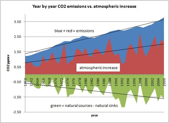
Compared with the growing natural sources of CO2, we observed: a decrease in sinks, or at least no increase:
The first graph is not up to dat, as the previous investigations show. The second graph is right: with the growing human emissions, the sinks are increasing too, so that the percentage of additional CO2 remaining in the atmosphere stays about the same, contrary to the expectations of CAGW people. Here a graph that shows that the sinks are increasing too:
Decrease in uptake by the oceans:
Especially the decrease in CO2 absorption by the ocean:
There is no decrease in CO2 uptake by the oceans, there still is an increase. From the link you provided:
Our results indicate that ocean uptake of anthropogenic CO2 has increased sharply since the 1950s, with a small decline in the rate of increase in the last few decades.
The rate of increase slightly decreased, but the uptake still increased.
There may be a decline in phytoplankton. But that simply is part of the total biosphere, which shows an increase in uptake…
Algae and bacteria may survive in Vostok ice at -40°C (that is the average temperature), but not more than that. Some even use CO2 for DNA damage repair, resulting in a drop of 0.1 ppmv CO2 reduction over 420,000 years… See:
http://www.pnas.org/content/101/13/4631.full.pdf especially item K. as that describes the pathway for survival in the Vostok ice core.
The protein has the ability to inhibit the recrystallization of ice
That is about the water internals of the microbe. If that would freeze, the cell would be dead. Nothing to do with the surrounding ice.
West Antarctica (Peninsula) and Greenland (edge) ice cores are not used for CO2 history, because the temperatures are not cold enough to prevent remelting in summer and algal/bacterial infuences neither are Greenland (summit) ice cores, because of acid + carbonate reactions caused by the deposit of volcanic dust from Icelandic eruptions.
The d13C decline in sponges:

More evidence of human induced CO2, absorbed by the oceans. The difference between the Atlantic and Pacific sponges is that there is much more deep ocean upwelling in the Pacific, which makes that the Pacific sponges are less fast declining in d13C and more irregular. See for a very long reconstruction (Bermuda):
The other article you linked to is for corals, which have a different methabolism, while coralline sponges directly reflect the d13C composition of the surrounding seawater.
d13C levels also are measured in ice cores air: very little difference in d13C over the Holocene, until about 1850:
http://www.nature.com/nature/journal/v461/n7263/full/nature08393.html
See further my comment on the historical data compiled by Ernst Beck:
http://www.ferdinand-engelbeen.be/klimaat/beck_data.html
Sorry that I answer so late, but “serious” response to Ferdinand Engelbeen requires analysis.
“… coccoliths will loose their shells with higher CO2.”
It should be noted – in the margin – that the evolutionarily – for millions of years – a mass of shells of single individuals – coccoliths species – continues to decline. Why? Eg: en eminent marine scientist from Poland, Professor K. Demel said: “Is calcium is an essential element for life, or whether it is a harmful element, the body hostile […]” that the body uses: “… only in the inlay, armor, shells and skeletons, and so additional creations, with an excess of calcium may even hinder the body’s vital functions [!].” (Demel, 1974.).
Dr Lough, eminent corals research, recently said: “Density bands show that coral growth and calcification on the Great Barrier Reef vary considerably over time.” “Coral records show that there have been several major increases and decreases over the past several centuries.“ “… the current decline appears to be a RETURN TO MORE NORMAL GROWTH CONDITIONS from high growth rates earlier this century”.
Indeed, but we also know that currently (since about 1990) the biosphere produces more oxygen than it uses. Thus the biosphere is a net sink for CO2 (the “greening earth”).
Of course it is!
It is beyond discussion. With a small “subject” for the last decade. “Terrestrial net primary production (NPP) quantifies the amount of atmospheric carbon fixed by plants and accumulated as biomass. Zhao & Running, 2010.
Biosphere is a net sink for CO2, but not the soil. The excess CO2 is from the soil – mainly arctic detritus. Its average age of a few thousand years (remainder), even more than 10 thousand. years (humus may be even older) – This is almost double the period of dissolution of 14C. So the CO2 from the “old stock” of soil, has the same isotopic composition as well as from fossil fuels. As for the oxygen – run “inventory” of soil CO2 is to provide an additional “raw material” for photosynthesis …
14C – its increase – it is, mainly, solar activity. (Eddy, 1976). Usoskin (usually: et al.) repeated for years: “The Sun spends ~3/4 of the time at moderate activity, ~1/6 in a grand minimum and ~1/10 in a grand maximum state. The modern solar activity is a grand maximum.”
Now I characterize soil respiration.
Tundra – Schlesinger (1991) and: Leith and Whittaker (19975) – the accumulation of C = 0.2 g/y C (very small – global), content C – 21.6 kg/m2 (highest – in global). On the website of Duke University writes: ”Lloyd and Taylor (1994 ) found that the relative sensitivity to temperature change is much greater for soils at low temperatures than for warmer soils. For example, in the absence of moisture limitations, an increase from 0 to 1 deg C would result in a 22% increase in respiration, while an increase from 25 to 26 deg C leads to a 5% increase. Thus, modest global change scenarios resulting in a 1 to 2 deg C increase in mean temperature would have the most significant effect on the 60 g C/m2 year respired by tundra.”
Bond-Lamberty and Thomson, 2010., and their comments:
“The increase in carbon dioxide given off by soils, about 100 million metric tons per year since 1989, won’t contribute to the greenhouse effect unless it comes from carbon that had been locked away out of the system for a long time, such as in ARCTIC TUNDRA [1 / 5 global land area] This analysis could not distinguish whether the carbon was coming from old stores or from vegetation growing faster due to a warmer climate. But other lines of evidence suggest warming is unlocking old carbon …”
“ Using the complete set of data collected from the studies, the team estimated that the carbon released in northern — also called boreal — and Arctic regions rose by about 7 percent; in temperate regions by about 2 percent; and in tropical regions by about 3 percent …”
“We estimate that the global RS in 2008 (that is, the flux integrated over the Earth’s land surface over 2008) was 98 ± 12 Pg C and that it increased by 0.1 Pg C yr-1 between 1989 and 2008, implying a global RS response to air temperature (Q10) of 1.5.” Only ?
Good and this. CDIAC: “The mean annual global soil-CO 2 flux over this 15-y period was estimated to be 80.4 (range 79.3-81.8) Pg C.”
I also recommend this comment by Alan Siddons:
High latitudes: Siberia – is warming up fastest. I propose this paper: Trends and uncertainties in Siberian indicators of 20th century warming. Esper et al., 2010.:
“… radiative forcing and associated feedbacks—is estimated at 1.5–4.5 °C…”
… and: Zone 64N-90N: “… the recent warming in this zone is over 5 °C per century!”
… and: Western Europe is warming much faster than expected, van Oldenborgh, 2009.
About what is happening in Siberia, and that in many areas there is dominated by natural variability, can be read here.
And how it affects the temperature of the soil?
Variations in temperature sensitivities of soil and microbial respiration: Implications for climate-carbon modeling, Suseela et al., 2010.: “Soil respiration is the largest flux of carbon dioxide to the atmosphere, releasing more carbon than fossil fuel combustion. Since temperature affects soil respiration, on a global scale, even a small warming-induced increase in carbon dioxide emission from soils could act as a positive feedback to climate change.”
Global pattern of temperature sensitivity of soil heterotrophic respiration (Q 10 ) and its implications for carbon-climate feedback, Zhou et al., 2009.: “Experimental studies of soil respiration have ubiquitously indicated that Q 10 has high spatial heterogeneity.” “However, most biogeochemical models still use a globally constant Q 10 in projecting future climate change …” “The mean Q 10 values for different biomes range from 1.43 to 2.03, with the highest value in tundra and the lowest value in deserts.” “The modeled heterotrophic respiration has a feedback intensity of 2.26 Pg C °C −1 , about 25% higher than that derived from a globally invariant Q 10 value.[…]”
Phytoplankton.
The comments cited authors by Boyce et al., 2010.:
“But their numbers have dwindled since the dawn of the 20th century, with unknown consequences for ocean ecosystems and the planet’s carbon cycle., … the global population of phytoplankton has fallen about 40 percent since 1950., That translates to an annual drop of about 1 percent of the average plankton population between 1899 and 2008., It’s very disturbing to think about the potential implications of a century-long decline of the base of the food chain …, They include disruption to the marine food web and effects on the world’s carbon cycle., Phytoplankton productivity is the base of the food web, and all life in the sea depends on it., Biggest declines at the poles, In addition to consuming CO2, phytoplankton can influence how much heat is absorbed by the world’s oceans, and some species emit sulfate molecules that promote cloud formation. [by the way, for me, this long-term trend – CLAW hypothesis – is the main cause of current warming – not: Svensmark’s theory, whether the changes in the electrical conductivity of the atmosphere, or of course – AGW].
Indeed, at least as fast as in the period 1975-2000.
Much more interesting is, however, the temperature drop in Europe. Between 1937(-9) and 194? it was the same, as the increase of temperature between 194? and 200? year!
The temperature drop in a few years (the interval between 5-10 years old) the same as “our” growth during the circa 60 years! Do not have a significant impact on the temperature of the water – especially the oceans NH – plankton?
The possible mechanisms of removal of CO2 by the oceans, we can read the example here: Glacial-interglacial atmospheric CO2 change: a possible “standing volume” effect on deep-ocean carbon sequestration, Skinner, 2009.
Thompson et al. in their work: An abrupt drop in Northern Hemisphere sea surface temperature around 1970, Nature, 2010.; for the years 1968 – 1972 – when the temperature drops in Europe was much smaller – say: “Here we show that the hemispheric differences in temperature trends in the middle of the twentieth century stem largely from a rapid drop in Northern Hemisphere sea surface temperatures of about 0.3°C between about 1968 and 1972.”
Here a graph that shows that the sinks are increasing too:
CDIAC “At the global scale, however, annual soil-CO2 fluxes correlated with mean annual temperature, with a slope of 3.3 PgCY -1 per degree Celsius.” Is it only?
Consider the “special cases” in the chart F.E. (referring to the fundamental work Sarmiento and Gruber, 2002). ENSO – El Nino – 5,5 ppm CO2 “permanently” add to the atmosphere. Year 1992 – a year after the eruption of Mt. Pinatubo. The amount of CO2, “added” to the atmosphere – about 0.5 ppm (5 times less than the average). Less sunlight – less photosynthesis – “green” sinks fall – CO2 is expected to increase. Decrease ocean temperatures, however – there is a greater absorption of CO2 by the sink. Assume for simplicity – “comfort” that the two sinks are in balance: the fall of one (biosphere) = increase in the second (oceans).
Why, then, decreases the amount of CO2 added (repeatedly) below average?
Simple, we did not include a major source of CO2. The decrease in temperature most inhibits the respiration of the soil.
Conclusion: The case of Mt. Pinatubo teaches us that the average proportion of anthropogenic CO2 in the so-called: unbalanced surplus in the atmosphere, can not exceed 1 / 5 of that surplus, ie – 0.5 ppm, and may be even smaller.
The average influence of temperature on CO2 levels is about 8 ppmv/°C for the ice ages – interglacials differences and MWP-LIA, 4 ppmv/°C for the variability around the trend (Pinatubo, ENSO).
However, according to Ensemble reconstruction constraints on the global carbon cycle sensitivity to climate, Frank et al., 2010.: “But themagnitudeof theclimate sensitivityof theglobal carboncycle (termed c), and thus of its positive feedback strength, is under debate, giving rise to large uncertainties in global warming projections.” “Here we quantify the median c as 7.7 p.p.m.v. CO2 per 6C warming, with a likely range of 1.7–21.4 p.p.m.v. CO2 per 6C.[ 1.28 or even 0.28 ppmv / ° C …]“ “Our results, based on the coupling of a probabilistic approach with an ensemble of proxy-based temperature reconstructions and pre-industrial CO2 data from three ice cores …” “Our results are incompatibly lower (P,0.05) than recent pre-industrial empirical estimates of 40 p.p.m.v. CO2 per 6C (refs 6, 7), and correspondingly suggest 80% less [!] potential amplification of ongoing global warming.”
Comparison of this work (based on ice cores), for example, Bond-Lamberty and Thomson, 2010, shows that the cores can not show the truth! Evidence of detail here is extensive, I promise that pass him within a month (maybe two …) for F. E.
Relying on ice cores so leads to conflicting conclusions.
The rate of increase slightly decreased, but the uptake still increased.
Why is the biosphere has not “kept pace” with the increase of soil respiration?
This paper: Knor, 2009., is for me – ecologist by population dynamics – very valuable. Shows the “middle phase” of a typical model of an oscillating – http://upload.wikimedia.org/wikipedia/commons/a/aa/Volterra_lotka_dynamics.PNG>Lotka–Volterra equation – “Population” of the victim (CO2 – soil respiration) – its growth is parallel to increased absorption of CO2 by the biosphere. It is a natural, typical, “ubiquitous” in the biosphere – the process.
And ends like this.
As for the “algae and microbes” in low temperatures – I promise a wider study (major items of literature I have over 100). Here, for the sake of discussion would note that according to: Does Algae Reduce the Ice Core CO2?, the main disposal of CO2 is where the ULV provides conditions for the algae to a very slow, but still, the development.
Also, I recommend (for starters): Bacterial Activity in South Pole Snow Is Questionable, and (particularly): Authors’ Reply (ibidem).
Here I would add only that the dust from above South America, always – not only in interglacial periods, reaching well over the entire Antarctic.
As for corals, sponges – as indicators of CO2, this is my adversary in Poland – AGW supporter, always adds the chart.
I am in a response (consistently), I suggest to him: comparison the papers: Rapid atmospheric CO2 changes associated with the 8,200-years-B.P., Wagner et al, 2002., fig 2., with fig. 3C (C4 %) in Comparison of multiple proxy records of Holocene environments in Midwestern USA, Baker et al. 1998,. And I then compile vectors, such as temperature, humidity, precipitation (which operate in opposite directions on the stomata of plants and the ratio of C3/C4), and concludes that the stomata and the ratio of C3/C4 plants, CO2 is only significantly – its concentration in the air. (PS: probably most accurately on the former p.CO2 “talks” C3/C4 ratio of the plant.)
A role for atmospheric CO2 in preindustrial climate forcing, van Hoof et al., 2008. a comparison of stomata – data – from ice cores. Here (stomatal index) there is not such a big difference in time between temperature and CO2, as in the case of work has already quoted Frank et al., 2010.: “The average correlation between individual temperature reconstructions and the mean CO2 record is 0.47 over the pre-industrial 1050–1800 period (all years are AD), increasing to 0.57 with a 50-year CO2 response lag—such timing is consistent with modelled CO2 response to a temperature step change.”
Although the stomata (from the nineteenth century) are usually dated by carbon 14 C with an average accuracy of + / – 35 years, according to me during the show further changes of CO2 than the cores. Rightly Wikipedia writes about the problems with dating of CO2 in the cores: “There are great problems relating the dating of the included bubbles to the dating of the ice, since the bubbles only slowly “close off” after the ice has been deposited.”
(I know the work of a new dating method of verification, but the questions are –CO 2 isotopes as tracers of firn air diffusion and age in an Arctic ice cap with summer melting, Devon Island, Canada, Clark et al., 2007. – one of the coauthors: Barnola)
Delta 13 C. On land, do not provide such results, as in the ocean. I will quote: A bi-proxy reconstruction of Fontainebleau (France) growing season temperature from AD 1596 to 2000, Etien et al. 2008.: Fig. 2 – there is a “severe” proxy delta – δ13C – The data d. 13C for the period under discussion (194? -5?) are slightly lower than for the late twentieth century, their decline as rapidly as in Beck and temperatures in Europe … Fig. 2. show several years of delay in the d18O – delta 13C. Of course, with these remarks: “correction for trends linked with anthropogenic carbon dioxide emissions; auto-correlation; strong inter-site variations and links with the number of beam samples (therefore reflecting strong inter-tree variability …”, “… 13C were not considered for past temperature reconstruction. [full agreement !]”
A propos Implications for coral-growth rates:
It is worth to consider that the final conclusion from this work: “There are multiple consequences of these findings for paleoclimatic reconstructions involving corals.”
Corals as indicators CO2. The graph of this work: Evidence for ocean acidification in the Great Barrier Reef of Australia, Wei et al., 2009., is no longer so obvious.
Stomata – are not confirm the figures E. Beck?
In this figure (Kouwenberg, 2005.) we can see (black line) a clear “hump” in the middle of the twentieth century.
At the end of it.
1. I can not find your answer -F.E., to respond to other significant “allegations” (compared with ice cores) in Ice Core CO2 Records – Geophysical Or Ancient Artifacts Atmospheres? – “allegations” (this time) is not provided by such: professor Jaworowski.
2. Ice cores, sponges, corals, cocoliths, such as ice cores are exposed to water and “life.” Water strongly influences the CO2 chemically “life” in the water are choosing coal 12C – even with the shell. For all these data sources, running the high pressure (also in the ocean – sedimentation). Professor Jaworowski always says: “… CO2 is 70 times more soluble than nitrogen and 30 times more soluble than oxygen” “Moreover, under the extreme pressure that deep ice is subjected to – 320 bars, or more than 300 times normal atmospheric pressure – high levels of CO2 get squeezed out of ancient air.”
3. The IPCC report says that data from the cores are “compatible” with data based on differences in the size of stomatal cells. Only that the latter, do not “talk” about the value of pCO2, but only about the course changes over time pCO2. Methane was to be further proof, but: Gases in ice cores, Bender, 1997.: “Finally, the CH4 concentration of the atmosphere was surprisingly variable during the Holocene.”
Me and Professor Jaworowski (yet separately), are preparing a new study on the cores – the ice and the bottom of the sea. In the next year (“how we’ll live”), “combine” their work (we regret that we can not do this together with E.G. Beck.) Your blog F.E., as well as discussions on other blogs (eg: Eli Rabett), research papers (eg: Z. Jaworowski: Ancient atmosphere — Validity of ice records, Oeschger, 1994.) are a source of extremely valuable information.
For today, we believe that the ice cores, “they say” only (in very, very approximate) of the changes of pCO2 in the atmosphere – at the time. Cores “do not say” practically nothing about “ancient” concentrations of CO2, because – of objective reasons, can not nothing “to say”, and therefore should never be used to create any theory – not just about global warming.
Well … there are two versions – a formatting error in “italic” – and such are the effects …
I would ask – if possible – to remove the other – a “new version” – in total, the first version is better formatted.
By the way, however, answer (right now – not a month or two …) a little bit more attention – I respond to one more the note F. E.:
”That is about the water internals of the microbe. If that would freeze, the cell would be dead. Nothing to do with the surrounding ice.”
Jean Brenchley, Research Summary:
“We explored the possibility that the historically prevalent climate conditions may have altered the microbial abundance and composition resulting in different diversity patterns. Because these results are important for determining whether in situ microbial metabolism could influence trace gases trapped in ice cores used to determine past climate records, we expanded these studies to include long term monitoring and detecting microbial activity of ice core samples and model organisms at sub-zero temperatures down to -32 o C.”
A bacterial ice-binding protein from the Vostok ice core, Raymond et al., 2008.:
“Here we describe such a protein from one of the Vostok ice core isolates and show how it might enhance survival under frozen conditions by affecting the physical structure of the ice […].”
“As shown in Fig. 1 d, RI activity could conserve the boundaries between ice grains in glacier ice. Such boundaries constitute a network of liquid veins that harbor microbial communities in sea ice (Deming 2002 ) and have been proposed as a microbial habitat in deep Antarctic ice (Price 2000 ). Triple junctions, where the boundaries of three ice crystal grains meet, are considered especially important as microbial refugia because of their greater liquid volume and tendency to accumulate ions and nutrients excluded from the ice (Price 2000 ; Mader et al. 2006 ). In fact, cultured cell suspensions of 3519-10 were found to accumulate at triple junctions when frozen under laboratory conditions …” “In the ice vein environment of glacier ice, microbes that do not produce an IBP could benefit from commensal relationships with species such as 3519-10, as has been observed in cold-adapted soil bacteria (Walker et al. 2006 ).”
“We have shown that a bacterium recovered from deep within the East Antarctic Ice Sheet possesses a protein with ice-binding activity that has sequence similarity to IBPs from species inhabiting other ice-bound habitats. These findings argue strongly that the strain is not a human- or laboratory-derived contaminant.”
I deleted the ‘newer version’ per your request.
221.A. Semczyszak said
December 8, 2010 at 6:28 am
Some answers to your objections…
– I think we agree that the “acidification” of the oceans is not a real problem, as coccoliths and corals did grow in CO2 atmospheres which were much higher during the Cretaceous when all these chalk layers were disposed…
Biosphere is a net sink for CO2, but not the soil. The excess CO2 is from the soil – mainly arctic detritus. Its average age of a few thousand years (remainder), even more than 10 thousand. years (humus may be even older) – This is almost double the period of dissolution of 14C. So the CO2 from the “old stock” of soil, has the same isotopic composition as well as from fossil fuels. As for the oxygen – run “inventory” of soil CO2 is to provide an additional “raw material” for photosynthesis …
I did use the word “biosphere” by purpose, as that includes net CO2 sinks (and thus oxygen producers) like plants and (land) algues and phytoplankton, but also net CO2 sources: microbes, yeasts, fungi and animals, including humans, which use the productivity of the former for food. That includes soil respiration. Soil respiration uses oxygen to “burn” carbon detritus in the soils. As the oxygen balance from fossil fuel burning shows a small deficit (at least in the period 1990-2003), all these natural sources and sinks together are a net source of oxygen, thus a net sink for CO2. Even if soil respiration increased 100% in the past 160 years and phytoplankton decreased 75% in the same period (which is not the case): that doesn’t matter, as the rest of the biosphere obviously more than compensated for the extra CO2 by increased growth…
14C – its increase – it is, mainly, solar activity. (Eddy, 1976). Usoskin (usually: et al.) repeated for years: “The Sun spends ~3/4 of the time at moderate activity, ~1/6 in a grand minimum and ~1/10 in a grand maximum state. The modern solar activity is a grand maximum.”
Agreed, but it is about the 14C DEcrease compared to what was expected from solar activity, which needed a correction for carbon dating…
Consider the “special cases” in the chart F.E. (referring to the fundamental work Sarmiento and Gruber, 2002). ENSO – El Nino – 5,5 ppm CO2 “permanently” add to the atmosphere. Year 1992 – a year after the eruption of Mt. Pinatubo. The amount of CO2, “added” to the atmosphere – about 0.5 ppm (5 times less than the average). Less sunlight – less photosynthesis – “green” sinks fall – CO2 is expected to increase. Decrease ocean temperatures, however – there is a greater absorption of CO2 by the sink. Assume for simplicity – “comfort” that the two sinks are in balance: the fall of one (biosphere) = increase in the second (oceans).
There is a quite nice correlation between the variability of the CO2 increase around the trend and global temperature: about 4 ppmv/°C. See: http://icecap.us/images/uploads/CO2vsTMacRae.pdf
Even a (moderate) warmer agrees with that, Pieter Tans, of the NOAA CO2 measurements, does attibute the variability to temperature and precipitation. See about half-way the .pdf:
Click to access tans.pdf
But that is about the variability around the trend (the derivative!). That doesn’t say anything about the cause of the CO2 trend itself. It is quite clear that the human use of fossil fuels is the cause, at least in the past 60 years: in no year there was any NET addition of CO2 from nature. 60 years long, nature as a whole was a net sink for CO2, not a source. Whatever the amounts circulating over the seasons. Whatever the changes in any individual release or uptake. Whatever the temperature influence may be…
Why is the biosphere has not “kept pace” with the increase of soil respiration?
This paper: Knor, 2009., is for me – ecologist by population dynamics – very valuable.
The Knorr paper confirms what I said: the increase of CO2 in the atmosphere is a fixed percentage of the human emissions: 55% of the emissions (land use changes not included) or 45% (land use changes included). With an incredible good correlation over the past 100+ years:

Far less convincing (including soil respiration) for temperature:

BTW: I am aware of the population “sawtooth” trends, was used in the firm I was working for to control the growth of salt crystals by controlling the % of “young” (small) crystals in a continuous reactor.
I am in a response (consistently), I suggest to him: comparison the papers: Rapid atmospheric CO2 changes associated with the 8,200-years-B.P., Wagner et al, 2002., fig 2., with fig. 3C (C4 %) in Comparison of multiple proxy records of Holocene environments in Midwestern USA, Baker et al. 1998,. And I then compile vectors, such as temperature, humidity, precipitation (which operate in opposite directions on the stomata of plants and the ratio of C3/C4), and concludes that the stomata and the ratio of C3/C4 plants, CO2 is only significantly – its concentration in the air. (PS: probably most accurately on the former p.CO2 “talks” C3/C4 ratio of the plant.)
One general remark: any data of CO2 or d13C over land have a lot of problems, as these are highly vulnerable to local/regional changes. These do reflect local CO2 levels and local d13C levels, not “global” changes. Only with a lot of these measurements on a lot of places, or with very huge (semi) global changes, one can have an impression of larger changes. That is one of the main differences with ice cores, which reflect global changes and coralline sponges, which reflect the changes in large areas of the oceans.
Wagner e.a. indeed may have indicated the rapid change caused by the Younger Dryas and the 8.2 kyr event. But the absolute level is questionable: the calibration occured over the 20th century against Mauna Loa + ice cores to remove the local bias over that century. But there is no reason to expect that the local bias didn’t change over the previous millennia. E.g. the oaks in The Netherlands used for calibration saw a change in landscape (and therefore regional CO2 levels…) from sea and marshes to polders and agriculture over the centuries in the main wind direction. Even periods like the MWP-LIA difference may have caused local CO2 trends to differ, as ocean currents (Gulf Stream) changed direction more southwards (Portugal, North Africa). Even the main wind direction may have changed then… Thus while the stomata (index) data are valuable because of their high resolution, take the absolute values with a grain of salt.
The same for land plants 13C/12C ratio: these reflect mainly local changes, including indirect temperatures due to changes in C3/C4 plant ratio. No direct correlation with CO2 levels, except an indirect correlation with fossil fuel burning in the past 1.5 century.
“The average correlation between individual temperature reconstructions and the mean CO2 record is 0.47 over the pre-industrial 1050–1800 period (all years are AD), increasing to 0.57 with a 50-year CO2 response lag—such timing is consistent with modelled CO2 response to a temperature step change.”
I had a direct discussion with Tom Van Hoof about his work, he had no response to the above objections against the stomata data. Further, the correlation between temperature (proxy via dD or d18O) and CO2 in ice cores is much more impressive:
http://www.ferdinand-engelbeen.be/klimaat/correlation.html
0.86 without lag, 0.87 with a ~600 years lag.
The dating of the gas enclosed in the ice cores indeed is a problem, as good as the resolution over longer periods back in time is. But that doesn’t change the reliability of the CO2 measurements themselves…
A propos Implications for coral-growth rates:
It is worth to consider that the final conclusion from this work: “There are multiple consequences of these findings for paleoclimatic reconstructions involving corals.”
Corals as indicators CO2. The graph of this work: Evidence for ocean acidification in the Great Barrier Reef of Australia, Wei et al., 2009., is no longer so obvious.
corraline sponges have less problems with this, as they reflect the d13C ratio of the surrounding seawater, without much interference of light or temperature. See http://www.agu.org/pubs/crossref/2002/2001GC000264.shtml unfortunately behind a paywall.
Stomata – are not confirm the figures E. Beck?
In this figure (Kouwenberg, 2005.) we can see (black line) a clear “hump” in the middle of the twentieth century.
That graph has only two points over the past century, derived from three (!) needles… But take the graph of the stomata calibration at:
http://www.pnas.org/content/99/19/12011.full Fig.1 or enlarged: http://www.pnas.org/content/99/19/12011/F1.expansion.html
The CO2 level around 1942 was 310 ppmv according to the Siple Dome ice core, 400 ppmv according to Beck’s analysis. The SI data show nothing special around 310 ppmv, while with 400 ppmv in reality, the SI index would be off-scale.
The article at:
http://hubpages.com/hub/ICE-Core-CO2-Records-Ancient-Atmospheres-Or-Geophysical-Artifacts
largely repeats the objections of Jaworowski, with some additions:
– Greenland ice cores have far more (volcanic) dust that Antarctic ice cores, therefore are less reliable than Antarctic cores for CO2 levels.
– Further a lot of “could”, “maybe”, “may influence”,… without any substance how much that may affect the CO2 levels…
If there was much migration, that would affect different ice cores at different rates, depending of accumulation, temperature, inclusions,…
But what we see is that ice cores with complete different circumstances show similar CO2 levels for the same ice age. Even more important: the temperature/CO2 ratio remains the same over the glacials – interglacials, each with 100,000 years further back in time. If there was migration or “squezing out” of CO2, the ratio would fade out over time.
Methane was to be further proof, but: Gases in ice cores, Bender, 1997.: “Finally, the CH4 concentration of the atmosphere was surprisingly variable during the Holocene.”
Yes it varied from 600-700 ppbv over the Holocene, after 1800 increased to 1500 ppbv and nowadays reaches over 1800 ppbv in direct measurements. Nothing to do with human activities, you think? See:
http://cdiac.ornl.gov/trends/atm_meth/lawdome_meth-graphics.html
Here we describe such a protein from one of the Vostok ice core isolates and show how it might enhance survival under frozen conditions by affecting the physical structure of the ice […].”
“As shown in Fig. 1 d, RI activity could conserve the boundaries between ice grains in glacier ice. Such boundaries constitute a network of liquid veins that harbor microbial communities in sea ice (Deming 2002 ) and have been proposed as a microbial habitat in deep Antarctic ice (Price 2000 ). Triple junctions, where the boundaries of three ice crystal grains meet, are considered especially important as microbial refugia because of their greater liquid volume and tendency to accumulate ions and nutrients excluded from the ice (Price 2000 ; Mader et al. 2006 ).
OK, even outside the microbe, but how far? sea ice is quite different from glacial ice. And depending on temperature, microbes hardly survive there, let be show much “life”, even if they survive… See Fig.1 of http://www.pnas.org/content/101/13/4631.full.pdf and point K. in the paper for Vostok. Based on the methabolism described there, the total use of CO2 for DNA repair of the microbes would be around 0.1 ppmv…
On acidification – I of course agree …
However, it will take to the reading of the proposed study (part I know) to add short for:
„that doesn’t matter”
This time, shorter: for the biosphere – certainly on a scale we observe the secular growth of the mainland – terrestrial – the mass – photosynthesis – probably to compensate (with allowance) decrease the possibility of the oceanic biosphere.
But we know – certainly – only that:
– The global balance of CO “go” on average 2 – 2.5 ppm “permanently” added to the atmosphere from circa 1958.
– Increases the share 12C, and decreases 13C and 14C, in atmospheric CO2.
– The biosphere – for at least the last 150 years, produces on average per year more oxygen than she could produce, if used only on average annually produced organic matter (contained in the distribution of CO2). It is beyond discussion. And only this.
It is different for the detritus, peat, humus – the “stocks” of organic matter – the old and very old.
The first assumption (AGW theory), it is here that the soil – a source of CO2 – is “zero”, or so little positive, that the biosphere is not only absorbs the excess soil, but even half of “our” sources CO2. In other words: after the removal of our source of oxygen for production of the biosphere could produce more than just its “current” production – produces oxygen net. Consumes more CO2 than it produces – including the stocks of soil.
The second assumption is that if the CO2 came from the biosphere – “kind of” decomposition of organic matter, it would indeed more 12C than, say, of CO2 from the ocean (though here we doubt), but not least 14C. The latter – 14C, could be less with only soil, but only if there have to use a really “old” inventory of soil – with a few, several thousand years. The current warming would be at least the same or greater (and faster) than those before the Medium Holocene Optimum – in one word: unprecedented – in size and violence. Such vehemence of the LIA is also leaving, however, show the work of von Storch’ example: here, and here, or Korhola.
And this is the problem to the dispute: the CO2 balance in the soil – the biosphere + stocks of organic matter from the past years. All references that I work on soil respiration, carbon cycle (even Frank et al., 2010.: 40% of the uncertainty related to projected warming of the twenty-first century [only twenty-first?] stems from the unknown behaviour of the carbon cycle …”) de facto, they say: CDIAC, a simplified model of Bern, etc.., may be confused and even a lot – when it comes to carbon balance. The uncertainty range is huge here.
For example, land. 11 the computer models, gave for 2,100 years (as projected in different p.CO2 for 2100 – 730 – 1020 ppm) results differ by up to circa 20 GtC/yr ! (Fig 1. (e), (f) – Climate–Carbon Cycle Feedback Analysis: Results from the C4MIP Model Intercomparison, Friedlingstein et al., 2006.).
J. Weiner, a Polish professor of a distinguished expert on the processes of decomposition, in the book: “Life and Evolution of the biosphere.” (Weiner, 2008.) writes: “There is no question about it, to the rate of decomposition of large areas could be measured from the satellite. Here you will get only information about the initial process of decomposition – studying evapotranspiration …”
– Adds: “… the issue of decomposition is not appreciated. The importance of primary production seemed to be obvious … … Decomposition of the problem remained fairly academic. Recently, however, it appears that a number of reasons the examination of decomposition become significant., … global climate change currently being observed can be related to changes in the carbon balance in the biosphere [….].”
Arctic, Siberian CO2 before 10tys. years (the “stocks” are huge) we are not able to distinguish from “our” – its chemical composition is absolutely identical to “our” – that is an important precursor of lignite.
The work that I cited (must admit that most very new – still requires discussion – the process of falsification, but …) have suggested that soil bacteria as a result of global warming have begun to use the current inventory of the thousands of years. One says that they do so from 1.8 million years – are responsible for past changes of CO2 in the atmosphere.
These works differ only in the assessment:
– First (and mainly) how more – how much;
– Secondly: if not ‘our’ emissions – an average of circa twice the unbalanced excess CO2 to be added to the atmosphere every year – the same soil respiration would also be the perpetrator of unbalanced surplus – if so, by how much she would be less – not “our” emissions?
1. As regards the “first”: The uncertainty range is huge, for example, in Bond-Lamberty and Thomson, 2010, is: + / – 12 Gt C per year (circa 2 times more than a year give “our” fossil fuels!). „However, the dynamics of RS are not well understood and the global flux remains poorly constrained.”
The increase in respiration per year (at least for the last decade) = 0.1 Gt C / year = growth rate of our, and by Alan Siddons: “On the other hand, since a 0.1 gigaton increase per year between 1989 and 2008 doesn’t square with a 10-15% total increase, perhaps the article is in error and the authors were misquoted.”
2. As regards the “second”: Working Knorr, 2009, showing a statistically steady increase in the biosphere from 1850 + Lotka–Volterra equation, shows that the biosphere acts as the “predator” – ie a long time, “do not eat” all of his victims, and a constant – a percentage of the. Without our surplus, probably by about 20-30% less (it should be calculated more accurately – I know) every year would be added to the atmosphere of CO2 from soil respiration – of course, until global temperatures to rise, or when the temperatures begin to fall, or would grow (or decreased) NPP.
Stomata regionally – it certainly does not work on them, the variability described by Massen – are too “stubborn”. Wagner, he tested its calibration later (2004). Especially comparison of Denmark gave America C3/C4 – randomness – regionality – similar changes in places thousands of miles away …
CO2 decides C3/C4? – I recommend for example: Climate and CO2 modulate the C3-C4 balance and _13C signal in simulated vegetation, Flores et al., 2009., Oligocene CO2 Decline Promoted C4 Photosynthesis in Grasses, Christin, 2007.
And according to skeptics such as I, the current temperature is rising due to unprecedented volatility of indirect solar activity: We are dealing here with the superposition of the Millennium cycles – the optimum (maximum forces) imposed at the time – aggregation – phase cycles: 2300 lat – magnetic activity Chaos and Intermittency in the Solar Cycle, Spiegel, 2009. and LNC (The 1,800-Year … + 6 000-Year; – perhaps unprecedented in the 12 thousand. years.
Also effect the unprecedented destruction of the ozone layer by the flashes of the sun and volcanoes – which react with a delay of high solar activity (the specific system it runs strong and very weak solar cycles 11-year-olds, such as: XI-XII, or: XIX-XX) – destruction of phytoplankton (mainly after the die near the pole and the equator) – CLAW and anti-CLAW theory + solar modulation atmospheric electricity („… greater than that of the cosmic ray chang.”)+ Svensmark theory. In total, this equates to: low a less clouds = warming – mainly in high latitudes, +the increase of the arctic soil respiration = a positive feedback (for warming) loop: the development of mankind – “our” CO2 …
Of course, it still must prove – and this should be addressed first of all …
I recommend – albeit written from the viewpoint of the theory of AGW supporter, but full of doubt, a very interesting study on the full spectrum of solar activity – including ozone are here: Solar Influences on Climate, L.J. Gray, J. Beer, M. Geller, J.D. Haigh, M. Lockwood, K. Matthes ,U. Cubasch, D. Fleitmann, G. Harrison, L. Hood, J. Luterbacher, G. A.
Meehl, D. Shindell, B. van Geel, W. White (Reviews in Geophysics, 2010).
Just a short addition:
Anticipating some objection to the claim that: it is the soil respiration may dominate the unbalanced “permanent” surplus CO2 in the atmosphere.
A few comments on the conclusions of this comment. I do not agree with most of the criticism of the work B.-L. – T. – contained therein, but:
“A 10 to 15 percent increase in CO2 emission from soils is 9.8 to 14.6 petagrams per year.”
Explanation: this does not mean that it has increased emissions by 10-15%. But that previous studies, models, not taken into account the amount of emissions from respiration.
Is this a significant difference, whether resulting from the “other techniques of calculation,” as want the authors to work?
Indeed, if the difference is significant, then the previous models (2006), which is based on assumptions CDIAC quoted here, did not include the 9.8 – 14.6 Gt C per year.
Virtually all of them assumed that, in the XIX – the beginning of the twentieth century, is the state equilibrium (or state close to equilibrium) in the natural carbon sources and sinks. Currently we have a surplus of natural sinks of natural sources. Just as the positive feedback, have experience in the rest of the XXI century (it was supposed imbalance) additional “revenues” of CO2 from the “nature”.
On the margins – “state close to equilibrium” and equilibrium, between “food” and that “what he eats” – in nature – is seen very rarely – and then only as a “temporary” – that is something extremely unusual in nature. As a rule, we are dealing with more or less deep and long-term imbalances.
Establishment by the creators of AGW theory, appearing for many years of close to a balanced, fluctuations of up to several ppmv of CO2, is from the perspective of population ecology – is extremely unscientific (against the amount of CO2 sources and sinks, and the strength of the main factors affecting them).
“… projected CO2 increase from the soils (0.1 Pg/yr) is around 1% of fossil fuel emissions (8 Pg/yr).” – the authors suggest. So, no problem. However, …
Circa 1950. was – 1.5 Gt C – Global Fossil Carbon Emission – to 2000 (7 Gt C) – was similar growth GFCE – also for the past 20 years. Difference 1950 – 2000 = 5.5 GtC 50 years = 0.11 Gt C / year growth GFCE … The increase in respiration during the last decades – is so similar, as increase GFCE – or higher (see below).
In addition, increase RS is, most likely – as it usually is: he could join at the beginning of an “exit” from the LIA – according to the L.-V. model, ie an increase in RS was earlier than the response of the biosphere and its prevalence has remained until now. To sum up: 0.1 Pg / yr could be compared with 8 Pg / yr, only if we assume a state equilibrium or surplus over the natural fluxes of natural sinks.
Suppose initially that there was an increase of RS 0.098 Gt C / year. If, however, the uncertainties surrounding the proposed B.-L. – T. (12 Gt C compared to 98 Gt C – 10%), it may also be less, and more. That’s why I stated in previous comments – the above – and I quote the work that helps to prove that probably need to add at least the 12 Gt C in the calculations B.-L. – T..
Eurekalert: Even soil feels the heat: “The regional data from the temperate and tropical climates produced results consistent with other results, such as more carbon being released at higher temperatures, but the boreal-Arctic climate data did not. In addition, removing only 10 percent of the boreal-Arctic data points was enough to invalidate the statistical significance of the boreal-Arctic result. Together, the results support the idea that more boreal data on regional climates is needed to reach statistical relevance.”
As for other claims, particularly the balance sheet – carbon cycle – discussion, because of the level of “uncertainty” – is open – I (and the ones who think like me) I (we)could be wrong …
P.S. Some of my comments (except for further reference – artificially creating a typical “cherry picking”) to certain websites are presented as an example of pseudoscience …
Well, where there are no scientific arguments, that there are always “other ways” to “discussion” …
By accident I deleted the comment on one sentence:
As for the content of oxygen in the atmosphere – it’s still very little precise quantitative indication (as compared to the huge difference between the concentration of O2 to CO2 in atmosphere) to recall the sentence proposed by the You paper , Bender, 2005.: “Calculations of interannual variability in land and ocean uptake are probably [?] confounded by non-zero annual air sea fluxes of O2. The origin of these fluxes is not yet understood.”
Probably the best all the problems with oxygen (and therefore APO), but still 13C, will show you the paper: Atmospheric oxygen and carbon dioxide observations from two European coastal stations 2000–2005: continental influence, trend changes and APO climatology, Sirignano et al., 2010.:
(It is true that this work relates to a particular period, but the problems may be common to different periods of time) “In the period from mid-2001 until mid-2005, we see an average increase of CO2 in the atmosphere of (1.7±0.2) ppm y−1, and a corresponding decrease of the airborne O2 fraction of (−20±2) per meg y−1, mainly caused by human activities, particularly fossil fuel burning. The major feature in the records is the fast decrease of the airborne O2. This decrease must be caused by an O2 sink up to now not accounted for. Two mechanisms have recently been proposed in the literature (Ciais et al., 2007; Randerson et al., 2006). An O2 decrease acceleration seems to have started during or shortly after the anomalously hot and dry summer in Europe of 2003. A relation between both is, however, still speculative, and the statistical base and significance are still small.”
“Extra input, in the form of fossil fuel CO2 measurements, is therefore needed. Radiocarbon measurements, eventually supplemented by CO concentration measurements with high timeresolution, could help to detect the fossil fuel fraction of the airborne CO2. This kind of observations is often associated to CO2 and O2 records (for example in the CarboEurope IP network, cf. http://www.carboeurope.org) and they could, therefore, help to remove the residual anthropogenic component from the APO derivation.”
4.A. Semczyszak said
December 10, 2010 at 11:08 am
It is different for the detritus, peat, humus – the “stocks” of organic matter – the old and very old.
The first assumption (AGW theory), it is here that the soil – a source of CO2 – is “zero”, or so little positive, that the biosphere is not only absorbs the excess soil, but even half of “our” sources CO2. In other words: after the removal of our source of oxygen for production of the biosphere could produce more than just its “current” production – produces oxygen net. Consumes more CO2 than it produces – including the stocks of soil.
The only difference between the oxydation of peat/humus and recent organic matter is the 14C content, which decreases over the millennia and is undetectable after some 60,000 years.
Anyway, the destruction of these carbon sources needs oxygen, as good as is the case for (relative) young carbon from leaves, stems and fallen trees. Thus the oxygen use determines if the biosphere as a whole is a net source or sink for CO2, including CO2 releases from soil bacteria, fallen leaves, animals and humans.
As we know with a reasonable accuracy the amount of oxygen used by the burning efficiency of different types of fossil fuels, it is possible to make the balance. That shows that the biosphere as a whole is a net sink for CO2, at least since 1990. Before that, the biosphere was possibly a slight net source, but we have no exact figures for the period before 1990.
While it is an extreme challenge of analytical skills to show the difference in oxygen trend in ppms, which is around 200,000 ppmv, it is made possible, be it with wide margins of error. These errors are not large enough to show that the biosphere is not a sink for CO2, even taking into account the possible error caused by the variability of the oxygen release/uptake from the oceans. Any such error only changes the partitioning between the biosphere and the oceans, but the total error in uptake of CO2 by the biosphere is +/- 0.6 GtC/year for a calculated uptake of 1.4 GtC/year.
Absolutely the last note (for me).
I think it is worth an interest in more recent literature – references – increasing doubt as to Your references cited by the IPCC report.
Certainly in the arctic soil is less 14C than in other soils. 10 thousand. years is not 60 thousand. – I agree, but …
I recommend a paper where Keeling is coauthor: Atmospheric 14CO2 Constraints on and Modeling of Net Carbon Fluxes 06-ERD-031, An LLNL Exploratory Research in the Directorate’s Final Report, Guilderson, 2009.. Here the “very old” coal Arctic is not discussed, only the “old” coal temperate soil – a source of atmospheric carbon 14C restored during the growing season – from the explosions of atomic bombs from the 60’s. This way you can reliably determine the respiration of soil zones: tropical, subtropical, temperate but not arctic soil …
And oxygen “behaves” so. With http://www.seafriends.org.nz/issues/global/climate4.htm>this remark: “ … the per meg delta value is not exactly the same as ppmv as it is based on the ratio of oxygen to nitrogen (21/78)=27% whereas oxygen ppmv is 210,000 (21%). The delta is calculated as in delta-O-13: deltaO2/N2 = ((O2/N2sample – O2/N2standard) / O2/N2standard) x 1E6, which is 30% higher than delta expressed as ppmv. Bender quotes a conversion factor of 4.8 from ppmv to per meg delta(O2/N2), which we don’t understand.”
(With this site I particularly liked this sentence: “… the origin of the diluting CO2 cannot be ascertained because the ocean’s outgassing is also poor in radioactive carbon.”)
About “manipulation” by oxygen, an unjustified assumption about the existence of natural balance, supplementary, can be read here: chapter: Oxygen Depletion & δ13C Lightening Do Not Match Human Activities, Glassman, 2010.
The change of oxygen concentration is not parallel to the growth of human CO2 emissions …
Test – “/i”
Test – “/em”
Test
7.A. Semczyszak said
December 13, 2010 at 8:23 am
From your reference:
O2/N2 ratios, a proxy for O2 concentrations, concurrently measured with CO2 concentrations, help determine regional CO2 fluxes by separating land fluxes from sea fluxes. Mace Head is the closest marine baseline station to Lutjewad, located at the same latitude, and therefore is taken as a reference.
This is the same problem as with the historical CO2 data compiled by the late Ernst Beck: local CO2 data over land can be used to determine the local fluxes, but not to determine (near) global CO2 levels. That is true for oxygen too: oxygen, nitrogen and CO2 are readily mixed in 95% of the atmosphere: all over the oceans and above a few hundred meters over land, but not in the first few hundred meters over land, where a lot of fast sources and sinks are at work. For that reason global CO2, CH4, O2 and N2O monitoring is done coastal (when the wind is from seaside) or on islands mid the Pacific.
If you want more detailed knowledge of parts of the carbon cycle, then measure in and over forests, near volcanoes or midst of land with tall towers… These are of interest for parts of the cycle(s), not for global monitoring.
9.A. Semczyszak said
December 13, 2010 at 3:04 pm
About the work of soil respiration by Ralf Keeling and others: again, this is looking at details of the carbon cycle, but again, that is of no interest for the global exchanges: oxygen is monitored at places which represent 95% of the atmosphere, not near ground in the residual 5% of the atmosphere over land.
There are several good points on the New Zealand website, but on other points they are completely wrong:
the CO2 hockey stick rests on a single ice core, ignoring centuries of chemical CO2 measurements.

only anthropogenic causes are considered (fuel gases, gases from living, gases from industry, land use), because “no other explanations could be found”
Well the “single” ice core was multiplicated:
Ice cores with different precipitation, temperature and salt/dust inclusions show the same CO2 hockeystick…
Other explanations were looked at, but all violate one or more observations. Only anthro CO2 fits all observations.
the CO2 absorption by terrestrial plants has been assumed to be constant, whereas plants grow faster in higher CO2 concentrations.
Who said that? Battle, Bender and others have shown that terrestrial plant growth is increased and that is even shown in the IPCC TAR as the “Bolin” graph.
By reading more at that site, I encountered so many errors, that it needs a whole website with many pages to correct them! Including:
– The false claim about “adjustment” of the gas age of Siple Dome to match the Mauna Loa data.
– The mixing up of residence time of CO2 in the atmosphere (about 150/800 = 5 years) and the excess decay time (4/800 = 40 years half life time).
– Their prediction that the oceans may be more important as sink/source, but that is based on an increase in temperature of half the deep oceans, while the thermocline of the oceans only contains some 1,000 GtC, somewhat more than the atmosphere.
– Based on solubility parameters of CO2 in seawater, the oceans are the cause of the increase. But the 13C/12C ratio of the oceans is too high and the pCO2 change of seawater is about 16 ppmv/°C, too small to explain the 100+ ppmv increase over the past 160 years…
– etc., etc.
the origin of the diluting CO2 cannot be ascertained because the ocean’s outgassing is also poor in radioactive carbon
That would be true if the CO2 circulation between permanent oceanic sources (equator) at upwelling places from the deep oceans and the sinks (mainly the NE Atlantic) did change substantially, for which there are no indications. But if that was the case, that also would increase the 13C/12C ratio, but we see a decrease.
The comments by Glassman:
The change of oxygen concentration is not parallel to the growth of human CO2 emissions …
Is entirely based on the digitizing of IPCC graphics, not on (available!) data. I have had several discussions with him on different topics, he hates scaling of items to show parallels (or not). I have less problems with that, as plotting on full scale sometimes hides relevant changes. But indeed, one need to look at the scale to be sure what is relevant and what not.
In this case, he expects a 1:1 use of oxygen for carbon when fossil fuels are used. But that isn’t right for oil (1.5:1) or natural gas (2:1)…
A similar problem with his dissection of 13C/12C ratio vs. human emissions: only one third of the calculated decrease in d13C shows up in the atmosphere, simply because the huge exchanges with the (deep) oceans (some 40 GtC/year) with a higher d13C ratio are thinning the decline:

10.curious said
December 13, 2010 at 3:43 pm
Test – “/i”
Test – “/em”
Test
Something goes wrong with the “closing” tags it seems: here a test of bold and italic:
bold
italic
this should be normal text
the closing tags don’t work, only a new tag overrules the previous tag(s).
Here again a test of italic:
italic
normal
italic
normal
Sorry for the tests, but indeed it seems now that all texts are italic, whatever tags one uses…
There you go. Someone messed up the italics.
“Only anthro CO2 fits all observations.”
1. Each natural carbon deriving from any “stock” before 1958, as well as reduces the amount of oxygen in the atmosphere during the period from 1958 to now. His age does not matter – counts is its quantity – the mass.
2. Oxidized carbon older than the period of disintegration of 14C – 14C reduces the concentration in the atmosphere – in the period after 18?? year, and certainly after 1958. Carbon from arctic soil is just as “out of balance” carbon, as carbon from fossil fuels – can not be treated as the carbon from other natural sources. Whether it has more than 5,000, or 5 (or even 50!) million years – does not matter. 14 C – in 10-12 thousand. year, decomposes at least 75%. On the other millions of years is only 25% … Carbon from no decomposed – for thousands of years – arctic remainder (remnants of the arctic lush life of the former Holocene optimums – usually ending in a rapid cooling of – lack of time to decompose) is 50-75% poorer in 14C than that of England or Poland soil …
And it is not finding the last “resort”- last chance by skeptics … but a fact.
3. I will not, “insisted, ” or other “space”, ways (other than combustion – carbon oxidation) the removal of oxygen from the atmosphere are well calculated. Range of error, however, be enormous – here I quote the website “seafriends”.
As for errors in quoted my side -“seafriends” – I agree – questions about O2/N2 contained therein, however, there are interesting and there is not full – the “good” response …
In the margin. CDIAC for accurate calculations of soil respiration – a margin of error – + / – – given the scale of uncertainty especially for the Arctic – tundra – are simply not serious.
Ferdinand Engelbeen – website: “CO2 science” attracted an enormous amount of literature on soil respiration and CO2 sequestration in the soil and biosphere – in order to prove that further warming will lead to the predominance of CO2 sequestration in the soil respiration. I fully agree with that, and I recommend You all to verify.
A team of “CO2 Science” I’ll want to submit for discussion a hypothesis: rapid exit from the LIA – an increase in arctic soil respiration = rising CO2 concentrations in the atmosphere (modified by rapid declines in SST and soil temperature on NH – that Beck’s research).
CO2 in the soil – heterotrophic bacteria – behave variably depending on the temperature – the temperature rise, first act positively, then negatively. With the increase in first is an increase in soil respiration followed: an increase in CO2 sequestration in the soil (…). Soil, warm parts of temperate zone, already accumulating more carbon than “burning”. Soil – depending on the temperature, can be source and sink for CO2 …
I recommend this paper for example:Thermal adaptation of heterotrophic soil respiration in laboratory microcosms, Bradford, Watts, and Davies, 2010. – It corresponds well with the previously cited work by me: A permafrost glacial hypothesis to explain atmospheric CO2 and the ice ages during the Pleistocene, Zech et al., 2010..
In the first cited the paper, I particularly recommend to discuss this sentence: “A future research priority is to evaluate the role that thermal adaptation plays in regulating heterotrophic respiration rates from field soils in response to changing temperature, whether seasonally or through climate change.”
Ferdinand Engelbeen – I do not want “to be right” and be “better in the discussion” – I suggest only interest in this “soil” hypothesis – and its up to verify the details. I think that it’s worth doing, and Your great knowledge – Ferdinand Engelbeen – can be found here “useful” (it’s not a compliment and: a statement of fact.) I believe that a detailed and accurate verification bet my thesis: It is mainly the soil – not “our” burning …, – this is not a “waste of time”. It is worth to do it.
(… and without accepting the work of Beck – the “soil” hypothesis simply “does not exist …”)
I propose to suspend the debate for a few months (let’s take the time to review the latest literature) on this – very welcoming – the website (I promise in the new year “more care” in formatting).
… and interactive discussion on the paper: Zech et al. 2010., is extremely interesting. Two reviewers assessed very negatively to this work, two others – can say: “enthusiastic” (…).
BTW this discussion is a lot of new (at least for me) work to explore – from the years 2009-10 – is often almost “completely” incompatible with each other – because virtually all based on ice cores (p.CO2) and the bottom of the ocean (in discussion shows there are problems with the Foramifera d.13C)?
Tundra and “her” carbon is still the great unknown …
Sorry but I need to (absolute!) end – for analysis – a propos of 14C: Decomposition of old organic matter as a result of deeper active layers in a snow depth manipulation experiment, Nowiński et al., 2010.: “Our results indicate that, as permafrost in tussock tundra ecosystems of arctic Alaska thaws, carbon buried up to several thousands of years ago will become an active component of the carbon cycle, potentially accelerating the rise of CO 2 in the atmosphere.”
… and tundra: Carbon respiration from subsurface peat accelerated by climate warming in the subarctic, Dorrepaal et al., 2009.: “Climate warming therefore accelerates respiration of the extensive, subsurface carbon reservoirs in peatlands to a much larger extent than was previously thought …” “Assuming that our data from a single site are indicative of the direct response to warming of northern peatland soils on a global scale [present global peat = 360 Gt C, remainder – 600-800 Gt C – in the LIA was probably much more], we estimate that climate warming of about 1°C over the next few decades could induce a global increase in heterotrophic respiration of 38–100 megatonnes of C per year. Our findings suggest a large, long-lasting, positive feedback of carbon stored in northern peatlands to the global climate system.”
Currently, as “mushrooms” appear in the work – papers of trying to explain the former changes of CO2 in the atmosphere. Hence I feel justified, if I add the latest evidence of the model oscillating L. – V.: Loss of Carbon from the Deep Sea Since the Last Glacial Maximum, Yu et al., 2010.. First, there are objections to 13C benthic: “However, existing deep-sea [CO3 2-] reconstructions conflict with one another, complicating paleoceanographic interpretations.”, but after: “Combined benthic δ13C and [CO3 2-] results indicate that deep-sea-released CO2 during the early deglacial period (17.5 to 14.5 thousand years ago) was preferentially stored in the atmosphere, whereas during the late deglacial period (14 to 10 thousand years ago), besides contributing to the contemporary atmospheric CO2 rise, a substantial portion of CO2 released from oceans was absorbed by the terrestrial biosphere.”
Current (LIA – modern time) to increase the surface free of ice in NH, it is not as spectacular as during the deglaciation, but the comparatively rapid. It is interesting that the terrestrial biosphere after circa 3 thousand. years, was able to “effectively” to respond to the increased concentration of CO2 in the atmosphere. Current surplus unbalanced, if not removed by the rapid cooling of the oceans, during the biosphere would probably removed by the secular scale.
237.A. Semczyszak said
December 23, 2010 at 7:53 am
1. Each natural carbon deriving from any “stock” before 1958, as well as reduces the amount of oxygen in the atmosphere during the period from 1958 to now. His age does not matter – counts is its quantity – the mass.
Agreed, but as the oxygen balance shows: the bulk of oxygen use is from burning fossil fuels. Only a small imbalance is from the total biosphere, including oxydation of carbon matter in melting permafrost. That imbalance was a small release of CO2 before 1990 and a more substantial (and increasing) uptake after 1990. Further, the mass balance shows that less CO2 is increasing in the atmosphere than fossil fuels are burned. Thus all natural sources and sinks together show a quite large deficit each year (currently 4 +/- 2.5 GtC/year). Thus whatever the natural sources (including volcanoes, warming oceans and permafrost) changed in the past 50+ (!) years, the natural sinks were larger.
2. Carbon from no decomposed – for thousands of years – arctic remainder (remnants of the arctic lush life of the former Holocene optimums – usually ending in a rapid cooling of – lack of time to decompose) is 50-75% poorer in 14C than that of England or Poland soil …
Agreed, but during the Holocene Optimum of some 6,000 years ago, more old 14C-free permafrost should have been decomposed than now, as the Arctic temperatures were higher than today, including the tree line far more North. If that had some important influence on the 14C/12C ratio, that would have been reflected in the carbon dating, but there were no troubles until about 1850. Since then the carbon dating needed some correction for the 14C/12C thinning, not in the earlier period.
The same for the 13C/12C ratio: an increased release of permafrost carbon would have decreased the d13C level over the Holocene, but that was not seen at all, to the contrary: the early Holocene shows an increase of d13C, as result of more uptake by the biosphere:
http://www.nature.com/nature/journal/v461/n7263/full/nature08393.html
3. I will not, “insisted, ” or other “space”, ways (other than combustion – carbon oxidation) the removal of oxygen from the atmosphere are well calculated. Range of error, however, be enormous – here I quote the website “seafriends”.
As for errors in quoted my side -“seafriends” – I agree – questions about O2/N2 contained therein, however, there are interesting and there is not full – the “good” response …
Battle and Bender calculated the error margin of the O2/N2 ratio measurements from the different stations as 1.4 +/- 0.8 GtC/year and 1.0 +/- 0.6 GtC/year for different periods. While the error margins are huge, even worst case, there still is an uptake of CO2 by the total biosphere, including CO2 releases from permafrost.
The NZ sea friends ( http://www.seafriends.org.nz/issues/global/climate4.htm ) are wrong on several accounts, including their oxygen balance:
There is something seriously conflicting here. Take the decade of the 1990s. During that decade humans burnt 65GtC or 30ppmv of which 57% or 17ppmv remained in air. During that same period, about 200 per meg = 200 / 4.8 = 41ppmv oxygen went missing, or nearly 2.5 times as much. We can account for 17ppmv oxygen but not for the remainder, a serious discrepancy. Why?
Some serious logic error here: the full 30 ppmv burned by humans uses oxygen, not only what remained in the atmosphere (much of the difference is absorbed by the oceans without influence on the oxygen balance) and not only 1:1 (for coal), but as their website also says, 1:1.5 for oil and 1:2 for natural gas, as the hydrogen content in the fuels also uses oxygen. Thus the full 30 ppmv fossil fuel CO2 needs more than 41 ppmv oxygen, the difference is what the biosphere produced as oxygen, thus the biosphere was a sink for CO2. See the Bolin graph for the period 1990-2000:

The other references you provided are for different individual carbon flows (including permafrost), which may be huge in flow and/or storage change over time, but that doesn’t matter at all, as we know the total carbon inventory for the atmosphere, very accurate over the past 50+ years thanks to C.D. Keeling, less accurate and smoothed, but still reliable, from ice cores over the past 800,000 years. And that shows that nature as a whole was a net sink for CO2 over at least 50+ years and probably the last 110 years.
This is an interesting article by David Middleton
http://wattsupwiththat.com/2010/12/26/co2-ice-cores-vs-plant-stomata/#comment-559354
Hi Tony,
In the article by Middleton, he thinks that stomata data (and Geocarb model data) are more reliable than ice core data. But that is very questionable: stomata data are proxies, not only influenced by CO2, but also by other items. And show local/regional CO2 levels, not background levels. While these can be calibrated against ice core (!) levels over the past century (+/- 10 ppmv), there is no knowledge of the influence of land changes in the main wind direction, nor changes of the main wind direction (and thus CO2 levels) itself over the previous centuries.
Ice core air bubbles, while smoothed, still contain the same composition as millennia ago, thus are direct measurements. Far more reliable than stomata data, but with a worse resolution the farther back in time. See further:
http://wattsupwiththat.com/2010/08/20/engelbeen-on-why-he-thinks-the-co2-increase-is-man-made-part-2/ about the reliability of ice cores.
and
http://wattsupwiththat.com/2010/09/24/engelbeen-on-why-he-thinks-the-co2-increase-is-man-made-part-4/ about where one finds “background” CO2 and further discussion of Beck’s historical data and stomata data.
Oh no! Not (yet) another ‘source of CO2 thread’. Please let it go Tonyb and Ferdinand and agree to disagree. People are either going to believe that adding CO2 to the atmosphere increases the concentration, or they are not. Another long thread will not change this.
Steve
I merely find it useful to gather the material in one place as this thread has become a good source of articles and comments-both pro and con.
Happy New Year Ferdinand!
tonyb
“… a good source of articles and comments-both pro and con.”
To this was to briefly describe the Mt. Pinatubo case (or 0.5 ppmv of CO2 added to the atmosphere in 1992) – which “speak” reference. The impact of EN(LN)SO (5.5 ppmv by 1998) well explains itself Beck (2008) – Evidence of variability of atmospheric CO2 concentration during the 20th century.
Do volcanic eruptions enhance or diminish net primary production? Evidence from tree rings, Krakauer & Randerson, 2003. :
“One hypothesis for this CO 2 anomaly is that since diffuse light is more efficiently used by forests than direct light, the increase in the diffuse fraction of sunlight due to scattering by volcanic sulfur aerosol in the years following the eruption substantially increased forest net primary production (NPP).” “Given that elevated aerosol levels and summer cooling last only ~2-3 years after an eruption, the persistence of declines in northern tree growth for up to 8 years after eruptions implies some additional mechanism that links these shorter-lived global eruption effects to sustained changes in tree physiology, biogeochemistry, or microclimate.”
The same is confirmed – says in this work:
Aerosols and the land carbon sink, Angert & Krakauer, 2010. in connection with (contra) to work: Impact of changes in diffuse radiation on the global land carbon Mercado, et al., 2009.
NPP compared with the CO2 to grow rats seen here, and here for zones.
Volcanoes – in total – so far the negative impact on global NPP – many years after the eruption (destruction of ozone?).
The resulting conclusions are most interesting in this paper: Impacts of large-scale climatic disturbances on the terrestrial carbon cycle, Erbrecht & Lucht, 2006. Every sentence is extremely important here:
“The amount of carbon dioxide in the atmosphere steadily increases as a consequence of anthropogenic emissions but with large interannual variability caused by the terrestrial biosphere.[…]”
“The response of soil respiration to changes in temperature and precipitation explains most of the modelled anomalous CO 2 flux.”
“We therefore conclude that during the last 25 years the two largest disturbances of the global carbon cycle were strongly controlled by soil processes rather then the response of vegetation to these large-scale climatic events.”
“Atmospheric carbon dioxide measurements show that the rate of increase of atmospheric CO2 varies substantially from year to year …” “It is widely accepted that these variations are caused by the terrestrial biosphere through the processes of carbon uptake during photosynthesis and carbon release during soil respiration …”
“In comparison, variations in the oceans [Two decades of ocean CO 2 sink and variability, Quéré et al., 2003.], deforestation, and land use change are much smaller …”
“Results show that a large fraction of the observed CO 2 growth rate variability is controlled by varying soil organic matter decomposition rather than changing plant productivity […].
And now my “right” of “riposte”…
Battle and Bender did not know that absolutely all of the current research emphasizes the possibility of a very large underestimation of CO2 from respiration in particular: “… from permafrost …” .
A significant drop (slow-out) of the surface permafrost, “1900 to 2100” – says the job: Sensitivity of a model projection of near-surface permafrost degradation to soil column depth and representation of soil organic matter, Lawrence et al., 2008.;
… and about rapid increases in permafrost temperature in this figure – notably the European part of Russia, is very interesting …
These in turn works show us how – to year 2008, was underestimated tank reservoir of carbon in the surface layer of permafrost: Soil organic carbon pools in the northern circumpolar permafrost region, Tarnocai et al., 2009.:
“In the northern permafrost region, organic soils (peatlands) and cryoturbated permafrost-affected mineral soils have the highest mean soil organic carbon contents (32.2–69.6 kg m −2 [!]).”Our estimate for the first meter [!] of soil alone is about double that reported for this region in previous analyses.”
“This 1672 Pg of organic carbon would account for approximately 50% [!] of the estimated global belowground organic carbon pool.[…]”
Vulnerability of permafrost carbon to climate change: Implications for the global carbon cycle, Schuur et al., 2008.: “We show that accounting for C stored deep in the permafrost more than doubles previous high-latitude inventory estimates, with this new estimate equivalent to twice the atmospheric C pool.”, ”The thawing of permafrost with warming occurs both gradually and catastrophically exposing organic C to microbial decomposition.”
“Agreed, but during the Holocene Optimum of some 6,000 years ago, more old 14C-free permafrost should have been decomposed than now …”
Unfortunately it is not so easy – in thawing present – current (and oxidised) permafrost meets surprisingly large proportion of the matter is earlier than “6,000 years ago” (Nowiński et al., 2010.: “Radiocarbon ages of heterotrophically respired C ranged from <50 to 235 years BP in July mineral soil samples and from 1,525 to 8,300 years BP [!] in August samples, suggesting that old soil C in permafrost soils may be metabolized upon thawing.”) – very depleted in 14C. Generally speaking: no oxidation of “straight” line – logarithmic decomposition is …
Oxygen – once again …
“For each 100 atoms of fossil-fuel carbon burned, about 140 molecules of O 2 are consumed. The surprise came when Keeling’s measurements showed that the rate of decline of O 2 was only about two-thirds of that attributable to fossil-fuel combustion during this period.” – that we know all of the textbooks (Broecker. The oxidation of organic matter is even greater oxygen consumption of carbon (not only: H but also for example, N, etc..) than burning fossil fuels …
… but the calculation of the deterioration of the oxygen content may be subject to considerable error. In addition to the above-cited problems with the appropriate measurements, there is the problem the same calculation. I recommend again:
Glassman : “The result is a mismatch with IPCC’s data at year 2003 by a difference of 1.3‰ [d13C], more than twice the range of measurements, which cover two decades.” “The CO2 added to the atmosphere is far heavier than the weight attributed to ACO2.”
“This circulation removes lightened atmospheric CO2, replacing it with heavier CO2 along many paths, some accumulated several decades to over 1000 years in the past. The mass flow model is a mechanical tapped delay line.”
Also, we do not know how much oxygen in the atmosphere comes from the ocean (range: 1 / 3 to ½ full). The problem of oxygen in the ocean is just tested.
So we know for sure that the oxygen content in the atmosphere is declining – how much and why? – it is “good ” question …
“… the early Holocene shows an increase of d13C, as result of more uptake by the biosphere …”
Of course, yes.
Cited by F.E. scientific work, however, says about 11 thousand. years ago (no deglaciation) and describes the oscillatory part of the model L – V, where the biosphere (after thousands of years) begins to “cope” with the excess CO2 and 12C of the deglaciation period, ie: 17.5 – 14 thousand. years (Yu et al., 2010.).
Apart from the novel hypothesis about the decisive role of permafrost – the soil in the Arctic p.CO2 increase during deglaciation – are well-established theories about the origin of CO2 is poor in 14C and 13C of the old carbon deep ocean.
For example, even the “press” reported the results of research: Ventilation of the Deep Southern Ocean and Deglacial CO2 Rise, Skinner et al., 2010.:
„We show that during the last glacial period, deep water circulating around Antarctica was more than two times older than today relative to the atmosphere. During deglaciation, the dissipation of this old and presumably CO2-enriched deep water played an important role in the pulsed rise of atmospheric CO2 through its variable influence on the upwelling branch of the Antarctic overturning circulation.”
The comments to the press for this paper:
“Scientists think more CO2 was locked up in the deep ocean during ice ages, and that pulses or ‘burps’ of CO2 from the deep Southern Ocean helped trigger a global thaw every 100,000 years or so. The size of these pulses was roughly equivalent to the change in CO2 experienced since the start of the industrial revolution.”
“As well as providing evidence for rapid release of carbon dioxide during deglaciation, the research illustrates how the ocean circulation can change significantly over a relatively short space of time.”
I recommend all the great scientific achievements L. Skinner.
I’ll add to it with the latest, for example:
Upper-ocean-to-atmosphere radiocarbon offsets imply fast deglacial carbon dioxide release, Rose et al., 2010. :
“The atmospheric decrease in the radiocarbon signal coincides with regionally intensified upwelling and marine biological productivity … …, suggesting that CO2 released by means of deep water upwelling in the Southern Ocean lost most of its original depleted-14C imprint as a result of exchange and isotopic equilibration with the atmosphere.”
Southern Ocean source of 14C-depleted carbon in the North Pacific Ocean during the last deglaciation, Basak et al., 2010.: “Our data exhibit a clear shift in the neodymium isotope values towards Southern Ocean values about 18,000 years ago, coinciding with the negative Δ 14 C excursion.”
… so that “seafriends” and E.G. Beck may be right that the ocean can be a significant source of the former and the current CO2 depleted in 14 and 13C – deep ventilation during El Nino (for example, from 1997/1998 …) has kept standards for d14c and d13C in the current climate.
1850 yr – but d13C – in a logarithmic – decrease from the Maunder Minimum …
I recommend here that the discussion before the year’s F.E. – the R.S.; about this post
Variability of leaf stomata – CO2 dominates at above 95% (eg, see above – a comparison with terrestrial d13C and C3/C4). This is a really great literature – references. Doubts to the ice core only is …
… and the work of the delay (250 years) in the reaction of CO2 to temperature is just great (Frank et al., 2010., or speak about the delay – 50 years) …
Steve Fitzpatrick
– I hope that within a few years – no longer a matter of “faith”.
And this We wish – ourselves – for the New Year.
”many years after the eruption” – sorry I give error link. http://earthobservatory.nasa.gov/Features/BorealThreshold/Images/uptake_temperature_rt.gif – it’s good link.
Even for the unconvinced – about the many possible explanations related to the decrease of oxygen in the atmosphere – and the importance of land-based sources of CO2 – a few sentences from the work Bender et al., 2005.:
“Interannual variability calculated from these data shows a strong land carbon source associated with the 1997–1998 El Nin˜o event, supporting many previous studies indicating that high atmospheric growth rates observed during most El Nin˜o events reflect diminished land uptake (which is not true because we now know that the 1997 land uptake increased rapidly) “. “Calculations of interannual variability in land and ocean uptake are probably confounded by non-zero annual [only annual?] air sea fluxes of O2. The origin of these fluxes is not yet understood.”
“Interannual variability in land biosphere and ocean uptake, calculated from O2 data, are compromised by ocean-atmosphere exchange.”
“The close coupling between total sequestration (calculated from the CO2 balance alone) and land biosphere sequestration (from CO2 and O2 constraints) between 1996 and 2001 validate earlier conclusions that high atmospheric CO2 growth rates during most El Nin˜o events are due to a large land source.”
That the claims of the cited work like this: “Nevertheless O2/N2 variations still retain an embedded signal due to variability in sequestration.” – have a “weak” basis.
246.A. Semczyszak said
December 29, 2010 at 10:21 am
To this was to briefly describe the Mt. Pinatubo case (or 0.5 ppmv of CO2 added to the atmosphere in 1992) – which “speak” reference. The impact of EN(LN)SO (5.5 ppmv by 1998) well explains itself Beck (2008) – Evidence of variability of atmospheric CO2 concentration during the 20th century.
Simply said, even with the Pinatubo eruption, the increase of CO2 in the atmosphere was fully attributable to the human emissions: humans emitted some 3.5 ppmv CO2 (7 GtC) into the atmosphere, of which 0.5 ppmv accumulated. The rest was absorbed by nature. Wherever that was and whatever the individual CO2 flows over the year, including what the Pinatubo and the permafrost or the oceans in some part emitted. Nature as a whole was a net absorber of CO2. Not a net source! See:

That is a question of mass balance: simple substraction of what is known as emissions and what is measured as increase in the atmosphere. All the rest is looking at partial flows, which may influence the total inventory at some point in time, but in the last 50+ years, nature was never a net source of CO2, always a sink.
Beck’s data are partially taken near huge local sources and local sinks over land these data are worthless for background CO2 levels. Historical data taken over the oceans or coastal with the wind direction from the seaside are more relevant (but still include severe measurement errors):

There are no historical data over the oceans in the “peak” period around 1942, but there is a simple proof about the reliability of the historical data: if there is a wide spread in the data, simply discard them, as that are data taken over land which have not the slightest resemblance to global CO2 levels…
Further, you cite a lot of partial comments from different sources, but out of context. While there is uncertainty in oxygen measurements, the trend since about 1990 is higher than the uncertainty, thus vegetation as a whole is a net sink for CO2, not a source, even if the emissions from permafrost might be elevated in the past decades.
All the rest is looking at partial flows, which may influence the total inventory at some point in time, but in the last 50+ years, nature was never a net source of CO2, always a sink.
– all the work – papers; I’ve quoted this statement partially or even completely undermine. Without our CO2 surplus would be only about 10-20% lower. The mass balance in the last half century has not been fixed – I repeat: “old carbon” was and is a non-balance sheet during the last 150 years, the amount was more than twice as underestimated, with CO2 respiration getting into the atmosphere – as well.
During the eruption of Mt. Pinatubo nature was “in retreat” – 1992 for 1997 – the indisputable fact – I’ll add more – the chart above – this slide: see on the second slide. Yes, we can say that nature in 1998, could go to zero …
… but for now “just good” we do not know sufficiently about the exact mass the biosphere.
A new satellites have yet to begin their study of the biosphere …
… these data are worthless for background CO2 levels …
– please read carefully the work of Massen and Beck, 2009. Accurate estimation of CO2 background level from near ground measurements at non-mixed environments.: “The CO2 versus wind-speed plot seems to be a good first level validation tool for historical data. With the required caveats it could deliver a reasonable approximation of past regional and possibly past global CO2 background levels.”
The last thing the fishes had to say was: ‘Thanks for all the plankton’.
H/t anna v.
=====
Supporters of the 100%-the years of our origin 2.5 ppmv CO2 – unbalanced annual average added to the atmosphere – in the last half-century – arguing: yet added to the atmosphere is just part of our emissions – our emission is circa 2 x greater than 2.5 ppmv of CO2 added annual average into the atmosphere. There is no place for another excess! If biosphere “can not cope” – is not able to “consume” all of our 5 ppmv of CO2, for example an increase of 5 ppmv of CO2 from soil respiration, ventilation of the deep ocean – if it actually existed – would lead to 7.5 ppmv CO2 unbalanced excess annual average. In other words, they assume that the growth of the surplus is almost straight (“uniformly accelerated”) in relation to an increase in CO2 sources, or only marginally logarithmic..
Skeptics (like me) think that this is not true. Along with the increased CO2 sources, the biosphere reacts in the shape of a logarithmic curve, or how they want supporters Gaia hypothesis – sinusoidal. What does this mean?
First a few words of introduction.
One of the circumstantial evidence that Formerly it was higher p.CO2 – than to “say” cores – is that the majority of optimum p.CO2 type C3 plants (plants with C3 photosynthesis respond fast to increased CO2) is 500-600 ppmv CO2, although some C3 plants have optimum even higher (even twice).
Always (optimum for C3) is at least 20% more than the current concentration of CO2. Up to 600 ppmv CO2 NPP is growing fast, perhaps even logarithmically – and “squared” x coefficient to determine the effects of other nutrients (in the margins: less than 150 ppmv CO2 C3 photosynthesis does not occur in practice.)
The concentration of CO2 in the atmosphere in the LIA was significantly lower than now (as it is confirmed that the cores, as well as stomata).
All also agree that the warming – out of the LIA – led to an increase p.CO2 – and increase NPP. There was an increase of soil respiration and ventilation of the deep ocean due to global warming – the linear (secular scale) out of LIA. This was the impulse for the biosphere.
Skeptics (like me), however, argue that the response of the biosphere (NPP) is logarithmic. Ie. if we assume that there was an increase of 5 ppmv – respiration, ventilation – (hypothetical value) per annum-in circa 300 ppmv (the beginning of the industrial era) – it removed the biosphere 3 ppmv from this source – a year. 2 ppmv CO2 is added to the atmosphere each year as “permanent” surplus.
Biosphere began to absorb more CO2 but according to the model of L. – V. – never all of excess – because the nature – photosynthesis tissue – always “has not kept pace” for the respiration of heterotrophic bacteria (ventilation of the deep ocean compared with the launch of the cork from the champagne). Nature can not keep up because: for example, had to – and must – come to replace: the permafrost – tundra – in the taiga. The advantage of the plant must obtain C3 – C4 on, etc..
However, there is the emergence of a new source of anthropogenic CO2 in the industrial era. New source – new 5 ppmv CO2 adds to the atmosphere – is to improve conditions for photosynthesis, the biosphere (as skeptics say like me) – and closer to the optimum of 500-600 ppmv CO2 – for C3. These “next” source so the biosphere reacts more positively than those earlier. These new – an additional source of absorption increases in NPP is not a 3 ppmv but about 4.5 ppmv. In other words, with an increase of CO2 sources for new 5 ppmv CO2, biosphere absorbs 3 ppmv growth with an increase in sources of CO2 by 10 ppmv – biosphere absorbs 7.5 ppmv increase from both sources. So net biosphere sink of CO2 (5 ppmv – an increase of respiration, ventilation – 7.5 ppmv increase in sinks – especially photosynthesis) – without an increase in CO2 from respiration but would not be 2 ppmv CO2 unbalanced excess CO2.
Gaia hypothesis proponents argue that with further increase in resources – ie, 5 ppmv of CO2 – the biosphere will have such a “luxury” conditions that not only consume the whole surplus, but also a portion formed from earlier sources.
In other words, a further increase in emissions ACO2 not only that it does not lead to an increase p.CO2, but it has lead to a balance – and even sinusoidal slight reduction – not only the unbalanced current excess, but also that of the twentieth century – as indeed is consistent with a model L.V.
In view of the huge range of variation regarding the growth of natural sources of CO2 – from the point of ‘momentary’ balance (the output of the LIA) – especially respiration (this increase it may be up to 3 – 4 times larger than our emission) – some (eg, a professor Jaworowski ), claim that our emissions is only 4% per annum in the atmosphere – as part of a permanently unbalanced excess.
Each add CO2 to the atmosphere more than 300 ppmv greatly increases the global NPP, but every drop p.CO2, below 300 ppmv – a fast decline in NPP. Thus, after the removal of “our” excess decrease NPP – photosynthesis – it will be much larger than the decrease of CO2 emission.
So say the skeptics like me – and it does not agree with AGW proponents – because that’s how a NPP in response to the rise and fall p.CO2 – this is another great (probably the largest and most important) area of the dispute.
AGW theorists argue that the biosphere for at least 50 years “can not cope” – with the increase of CO2 sources at the beginning of (the output of the LIA), the percentage absorbed more CO2 than with further increase in volume of CO2 sources – if there were only the natural sources of CO2 – the biosphere would be in equilibrium: sources = sinks.
Proponents of AGW theory , say also: to a fall in alkaline ocean – for example, there is deficiency of nitrogen, calcium, iron – oceanic photosynthetic potential can not be realized – and higher temperatures reduce photosynthesis on land.
Briefly about the lands: more efficient photosynthesis takes place at higher temperatures – see figure here. Higher temperatures are also more terrestrial aerosols ( isoprene) more diffused light – the increased efficiency of photosynthesis. Commentary on the figure quoted above is as follows:
“The upper curve is the same for C4. From this it is clear that at double CO2 concentration, not only has the efficiency of C3 crops improved tremendously, but the temperature at which optimal photosynthesis occurs in C3 increases up to that of C4. Thus the vast majority of food crops will benefit hugely by increased CO2, and even more so by increased CO2 coupled with warming”
Tissue terrestrial plants – despite the huge variation in the growing season – in the longer term react slowly to changes in CO2 as compared with single cell – the majority – the huge potential of photosynthesis (a relatively small weight) of the biosphere oceans. Here you can increase NPP depends mainly on the amount of CO2 – the skeptics say …
… and have the evidence:
Enhanced biological carbon consumption in a high CO2 ocean, Riebesell et al., 2007. :
“Here we show that dissolved inorganic carbon consumption of a natural plankton community maintained in mesocosm enclosures at initial CO2 partial pressures of 350, 700 and 1,050 atm increases with rising CO2. The community consumed up to 39% more dissolved inorganic carbon at increased CO2 partial pressures compared to present levels, whereas nutrient uptake remained the same.”
Ca – by website “seafriends” – dr. A. Floor:
“But the concentration of Ca (411ppm) is 10.4 mmol/l and that of all CO2 species (90ppm) 2.05 mmol/l, of which CO3 is about 6%, thus 0.12 mmol/l. Thus the sea has a vast oversupply of calcium. It is difficult therefore to accept that decalcification could be a problem as CO3 increases. To the contrary, it should be of benefit to calcifying organisms. Thus the more CO2, the more limestone is deposited. This has also been borne out by measurements (Budyko 1977).”
N – nitrogen.
I quote from my work – review (partly available on the Internet only as comments):
“In this pH range:
– Trichodesmium have maximum atmospheric N2 assimilation,
– do not having denitrifications (Michael H. Huesemann w „The inhibition of marine nitrification by ocean disposal of carbon dioxide” (2002).
… about one – Scientists’ from Leibniz Institute for Marine Sciences in “Effect of rising atmospheric carbon dioxide on the marine nitrogen fixer Trichodesmium”, said:
“As Hutchins et al . [2007] describe it, their work revealed that at atmospheric CO 2 concentrations projected for the year 2100 (750 ppm), “N 2 fixation rates of Pacific and Atlantic isolates increased 35-100%, and CO 2 fixation rates increased 15-128% relative to present day CO 2 conditions (380 ppm).” And in what they call one of their “most striking results,” they found that “increased CO 2 enhanced N 2 and CO 2 fixation and growth rates even under severely phosphorus-limited steady-state growth conditions [our italics].” They also report that “neither isolate could grow at 150 ppm CO 2 ,” but that “N 2 and CO 2 fixation rates, growth rates, and nitrogen: phosophorus ratios all increased significantly between 380 and 1500 ppm,” and that “in contrast, these parameters were affected only minimally or not at all by a 4°C temperature change.” In discussing the implications of their findings, Hutchins et al . note that current global estimates of N 2 fixation by Trichodesmium are about 60 x 10 9 kg N yr -1 , and that if their experimental results can be extrapolated to the world’s oceans, by 2100 this amount could increase to 81-120 x 10 9 kg N yr -1 . In addition, they say that “if these estimates are coupled with modeling predictions of a 27% warming-induced expansion of suitable habitat (Boyd and Doney, 2002), calculations suggest that global N 2 fixation by Trichodesmium alone could range from 103-152 x 10 9 kg N yr -1 by the end of this century,” which is to be compared to recent estimates for total pelagic N 2 fixation of 100-200 x 10 9 kg N yr -1 (Galloway et al ., 2004).”
For this we should add that – besides very poor – huge areas of ocean are extremely rich in iron …
The positive effect of a decrease alkaline oceans could argue for hours …
So I will cite only dr A. Floor – comments oceanic map pH : “Note that upwelling [it is most high NPP in all oceans] areas are more acidic because high-CO2 bottom water surfaces, warms up and makes CO2 more readily available, a bonus for photosynthesis by marine plankton.”
At the end, however, I must agree with the final conclusion from this work – Counterintuitive carbon-to-nutrient coupling in an Arctic pelagic ecosystem, Thingstad et al., 2008. : “Our results highlight how descriptions of present and future states of the oceanic carbon cycle require detailed understanding of the stoichiometric coupling between carbon and growth-limiting mineral nutrients in both autotrophic and heterotrophic processes.”
Counterintuitive carbon-to-nutrient coupling in an Arctic pelagic ecosystem, Thingstad et al., 2008.
About Roy Spencer’s articles:
I have responded on his first article (about the d13C changes “proving” that the oceans were the main source). He published that on his web site too:
http://www.drroyspencer.com/2009/01/the-origin-of-increasing-atmospheric-co2-a-response-from-ferdinand-engelbeen/
But I was not aware of the newer article of may. The basic error is that he looks at the cause of the variability in the rate-of-change not of the change itself. And as already agreed, the variability in rate of change may be caused for 80-90% by temperature. That has nothing to do with the change itself, which is 95% caused by the emissions. Temperature plays hardly a role on longer term (8 ppmv/°C).
I have read the work of Massen and Beck, 2009 very carefully. While it is a good approximation, one need accurate measurements (of which I have my doubts for Giessen) and one need enough datapoints at over 4 m/s wind speed (only 20 datapoints in Giessen). Thus unfortunately the Massen/Beck method is not applicable for the main dataset where the peak of 1942 was based on. Moreover, at the other side of the ocean, average data (within vegetation) show 250 ppmv, much too low, but as (in)valid as these from Giessen.
Skeptics (like me) think that this is not true. Along with the increased CO2 sources, the biosphere reacts in the shape of a logarithmic curve, or how they want supporters Gaia hypothesis – sinusoidal. What does this mean?
Nature as a whole reacts to increases in the atmosphere in the same way as any simple first order process reacts to a disturbance: if you add some extra CO2 (whatever the source), the process tries to reduce the disturbance. If there was a one-time extra shot of CO2, the extra would go down in a logarithmic way, with a constant emissions, that would lead to a higher level which is reached assymptotically and as the current emissions are steadily increasing, the levels in the atmosphere (and the sinks) are steadily increasing too.
Nature can not keep up because: for example, had to – and must – come to replace: the permafrost – tundra – in the taiga. The advantage of the plant must obtain C3 – C4 on, etc..
But it did keep up: the increase in the atmosphere caused higher levels which at a certain moment are again in equilibrium with the biosphere and the cooler ocean parts. This is seen in all Antarctic ice cores (including the high resolution Law Dome ice cores) as a 6 ppmv higher CO2 level after the LIA, for an app. 0.8°C higher temperature. Thus the natural temperature – CO2 ratio is about 8 ppmv/°C when a (dynamic) equilibrium is reached.
Gaia hypothesis proponents argue that with further increase in resources – ie, 5 ppmv of CO2 – the biosphere will have such a “luxury” conditions that not only consume the whole surplus, but also a portion formed from earlier sources.
I don’t know where that is based on. The graph you provided shows an increase of 30% for 100% more CO2, that is an increase, but not “consuming the whole surplus”. Only with (much) higher temperatures, photosynthesis may reach 100%. And only if the emissions are below the sink rate, then we will see a downgoing CO2 level…
Here we show that dissolved inorganic carbon consumption of a natural plankton community maintained in mesocosm enclosures at initial CO2 partial pressures of 350, 700 and 1,050 atm increases with rising CO2. The community consumed up to 39% more dissolved inorganic carbon at increased CO2 partial pressures compared to present levels
Thus plankton uses 39% more CO2 for a 300% CO2 level in the atmosphere! Still far from catching up with the atmospheric increase…
I do agree that an increase of CO2 is positive in almost all cases for plant growth, but still, the increase is 95% caused by the emissions (and maximum 5% by the temperature increase since the LIA).
and maximum 5% by the temperature increase since the LIA
I agree …
1. E. G. Beck – the end (above), “he insisted”, however, that in his new paper will present evidence of the indisputable increase of CO2 in the 30-40’s of the twentieth century. Massen writing a paper of Beck agreed with the possibilities of validation of historical measurements of CO2.
2. I do not agree with the hypothesis of Gaia (at least not with such a fast response of the biosphere) – I gave as an example the possibility of changes in the interpretation of sources – sinks – the lack of a simple mass balance.
I believe that the simpler explanation – the increase in natural sources by orders of magnitude larger than the estimated 8 ppmv / ° C (based on it – 8 ppmv – some models assume that our surplus will be removed only by the biosphere for more than: n x 10 thousand years.! ), should be enough. Then – for example, of 80 ppmv of the hypothetical natural growth of a source / ° C – out of the ocean biosphere + removes 78 ppmv, and our average of 5 ppmv for the last fifty years – 4.5 ppmv. In this model, the biosphere may feel even less responsive to a new source of CO2, than it appeared from the optimum of photosynthesis.
Of course, these 80 ppmv CO2 you need to prove – is I know. For starters, you need to prove that it is at all possible. However, a simple mass balance that assumes that if there was a natural surplus is “ours” would be added to the whole atmosphere – it is untrue – a new source is a new positive impulse for the biosphere – is this we agree. Work of Spencer (and practically all of my citation) demonstrates, above all, that natural variations of sources and sinks (year on year) of CO2 are higher than emissions from burning fossil fuels. Other conclusions must be proved – is fact.
Reflecting on the value that should be adopted for the calculation of natural sources of growth since LIA – I went back to interactive reviews paper – and paper itself Zech et al. 2010.:
“Major implications of our study also arise for our understanding of the role of high
latitude regions for the carbon cycle today.” “We acknowledge that part of the total carbon inventory at high latitudes accumulated only since the Holocene, but (i) non-glaciated permafrost regions likely had very different carbon dynamics than formerly glaciated areas, in which many peatlands developed after deglaciation …”
“This feedback would likely have continued during the Holocene, had there not been man-made global warming and increasing anthropogenic emissions (Ruddiman, 2003), reaching _5 Pg/year during the last century. To put this emission rate into context, the positive feedback due to thawing permafrost now is _1 Pg/year (Schuur et al., 2008; Tarnocai et al., 2009), while the natural rate of permafrost carbon release during the last deglaciation (1000 Pg over 5 ka) can be estimated to have been only _0.2 Pg/year. We are thus responsible for rapid and probably unprecedented rates of climate and environmental changes in the Arctic.”
1 Pg C (Pg C = Gt C) 1 has to be added over the next 40 years, even though we know that the last sentence of Zech et al. is likely to be untrue. F.E. – You has already written a clearly about further to the north border of the forest six thousand. years ago. Paper Astrid Lysa by 2008 years Less ice in the Arctic Ocean 6000-7000 years ago, does not leave doubt as to the absence of the abovementioned “unprecedented rates “, and me – as usual – in the context of this work are reminded (again) work Evidence of 6 000-Year Periodicity in Reconstructed Sunspot Numbers, Xapsos and Burke, 2009.: “We have examined these data using Hurst analysis, a moving average filter, and Fourier analysis. All of the procedures indicate the presence of a long term (≈6 000 year) cycle not previously reported.”
So those old “0.2 Pg / year” “over 5 ka “obtained on the basis of ice core proxy …
In a review Zeng N. writes about the origin of carbon sources: “For example, (a) land carbon change in non-ice/non-shelf region is about 200 GtC, dominated by cold regions (b) He simulated a transient d13CO2 at deglaciation which offers even a more nuanced picture, but consistent with the hypothesized land carbon change. (c) He estimated a 100-200 permill anomaly in C14 due to the release of ancient land carbon.”
I’ll quote – an analysis of G. Munhoven (Referee) – a review work Zech et al. and Interactive comment on “A permafrost glacial hypothesis to explain atmospheric CO2 and the ice ages during the Pleistocene” by R. Zech et al.:
“… the carbon stock in terrestrial soil and vegetation increased by 750–1900 PgC during the deglaciation, with permafrost generally not considered; (2) vegetation model results provide estimates of 600–1100 PgC for this increase, also lacking explicit representations of the peculiar permafrost soil dynamics; (3) the marine carbon isotopic data suggest a lower net transfer of only 300–700 PgC of organic carbon from the combined ocean+atmosphere to the land reservoirs (vegetation, soil, permafrost, . . . ), and, if corrected for a possible fractionation related to changing carbonate ion concentrations in the ocean between glacial and interglacial times, these estimates may at worst reduce to zero. [?!]”
Do we even know – what do we really know? Over 1000 Pg C (with only the permafrost) may behave very differently depending on very many – do not quantify well even initially – factors. Our CO2 added is the atmosphere during the 150 years from the combustion of fossil fuel + cement – is circa 350 Pg C. With the change in land use 500 Pg C.
“Both estimates are converted in terms of their potential effects on atmospheric CO2 (increases by 150 ppmv and 500 ppmv, resp.). Although arithmetically correct these effects do not have any significant meaning: the at first impressively looking increases in atmospheric pCO2 are going to be reduced by a factor of ten as a result of ocean uptake; the actual maximum increase will depend on how fast that carbon would be released.”
“For 1000 PgC released into the atmosphere from permafrost soil, 600 PgC are taken up by the rest of the terrestrial biosphere, 400 PgC are thus left in the atmosphere, 360 PgC of which are absorbed by the oceans on time scales of a few thousand years, leaving 40 PgC in the atmosphere (i.e., 19 ppmv – with the 850 PgC terrestrial biosphere regrowth, only 15 PgC would be left in the atmosphere, i.e., 7 ppmv), simply as a result of ocean chemistry and carbonate compensation, without any change in any oceanic process. Changes in oceanic processes are then required to pump 160 PgC into the atmosphere in order to produce the net 200 PgC increase observed. There is no other reservoir left that could possibly fulfil this role.”
So without the oceans we will not give you advice here …
“There is no justification for revising the role of the ocean in explaining glacial-interglacial pCO2 changes in the atmosphere: ocean based mechanisms appear to be required to provide 80%, possibly even more than 90% of the total net glacial-interglacial pCO2 change, even if the permafrost storage change estimate of 1000 PgC of Zimov et al. (2009) is taken at face value.”
“Even if there remain uncertainties regarding the amplitude of glacial-interglacial changes of the global mean _13C in the oceans, the sign of the change appears to be robust: the oceans had a lower _13C at the LGM than during the Holocene. This provides a constraint on the glacial-interglacial transfer of carbon depleted in 13C between the ocean+atmosphere and land reservoirs, that may not be simply dismissed.”
Today, however, the ocean absorbs only circa 40% of total surplus of sources over sinks …
Relying on the cores very limited opportunity to explain changes in the reservoirs of carbon (as there is the ocean biosphere must be “crazy” speed up or slow down), the more that the author reviews Munhoven, makes yet another important source of CO2 during warming.
In paper Holocene carbon cycle dynamics, Kleinen et al., 2010. :
“Ice core data of atmospheric CO 2 between 8 ka BP and preindustrial climate can only be reproduced if CO 2 outgassing due to shallow water sedimentation of CaCO3 is considered. In this case the model displays an increase of nearly 20 ppmv CO 2 between 8 ka BP and present day. Model configurations that do not contain this forcing show a slight decrease in atmospheric CO 2. We can therefore explain the late Holocene rise in CO 2 by invoking natural forcing factors only, and anthropogenic forcing is not required to understand preindustrial CO 2 dynamics.”
Despite the introduction of this source: “The model is able to simulate the return of CO2 concentration to its interglacial value after termination of the glacial cycle but simulated CO2 concentration still lags considerably behind the ice core reconstructions.” (Simulation of glacial-interglacial atmospheric CO2 variations using a comprehensive Earth system model of intermediate complexity, Brovkin et al., 2010.)
I tried to also find the work of a global balance of oxygen beyond the work: Bender et al., 2005. and objections to the validation measurements N2/O2.
In addition to the work of “daunting” anoxia (fall in oxygen uptake by the ocean as a result of AGW), I found: A conceptual model for the temporal spectrum of oceanic oxygen, Ito and Deutsch, 2010.: “Observed across the world oceans in recent decades have been interpreted as a response of marine biogeochemistry to climate change. Little is known however about the spectrum of oceanic O2 variability […].” “We find a statistically significant spectral peak at a 15–20 year timescale in the subpolar North Pacific [background], but the mechanisms connecting to climate variability remain uncertain.”
Whit old papers: On evaluating ocean models with atmospheric potential oxygen, Naegler et al., 2006.:
“We used observed and simulated atmospheric potential oxygen (APO) to evaluate simulated air-sea flux fields from 11 ocean global carbon cycle models. APO is defined in terms of atmospheric CO2 , O2 and N 2 so as not to depend on terrestrial photosynthesis and respiration. Hence, it is in principal suited to evaluate simulated air-sea fluxes of these gases.”
“The simulated amplitude of the seasonal APO variability was generally less than observed. We conclude that it is difficult to validate ocean models based on APO because shortcomings in atmospheric transport models and problems with data representativity cannot be distinguished from ocean model deficiencies.”
Mass balance, D13C, D14c, p.O2 are no barrier to indicate the natural sources of CO2 – a major source of surplus p.CO2 unbalanced current in the atmosphere – or the accuracy of the data from ice cores, stomatal and historical measurements. The obstacle is to determine real size of the sources and sinks. Furthermore, if it were otherwise there would be no skeptics among scientists.
As long as we do not will determine the actual size of reservoir C (and flows between them), with an error not exceeding the allowable limit – it is the old arrangements (IV IPCC) is often very detailed (and now so widely disputed) can not form the basis of evidence “for and against” .
The latest version of the report being prepared IPCC I would agree only with those conclusions (well, that they appeared):
“Ice core data indicate that CO 2 varied within a range of 180 to 300 ppm and CH 4 within 320 to 790 ppb over this period [of the last 650 kyr]. Over the same period, antarctic temperature and CO2 concentrations covary, indicating a close relationship between climate and the carbon cycle.”
“It is very likely that glacial-interglacial CO2 variations have strongly amplified climate variations, but it is unlikely that CO2 variations have triggered the end of glacial periods. Antarctic temperature started to rise several centuries before atmospheric CO2 during past glacial terminations.”
TonyB,
for the archives, here is another theory for disturbance of Antarctica:
http://www.bibliotecapleyades.net/antarctica/antartica24.htm
8>)
To Tony –
I am very appreciative that on my blog you pointed out to me this post here. It is always reaffirming to see that something I focused on is supported by so much background. Don’t we all love it when we see our good judgment confirmed?…LOL
Actually, I am amazed that I did not actually post on this at my blog. I had a draft ready since two months ago. I wrote about how Callendar cherry-picked his data in his 1938 paper and how Slocum in 1955 called him out on it. I just posted it.
The eminent Thomas Huxley having values of 327-380 should argue loudly for Callendar’s 1938 and 1958 papers to have been seriously flawed, if not outright fraudulent In claiming a 290 ppm value for the pre-1900 period (which some now even fudge downward another 10 ppm to 280 ppm).
Huxley’s values are certainly confirming of Slocum’s work – and Huxley’s values as of 1883 are generally even higher.
* * * *
FYI: The Thomas Huxley book “Physiography – An Introduction to the Study of Nature (1883)” is available in its entirety at http://tiny.cc/btx7aw.
Steve Garcia
Hahahahahaha –
I love it.
This is exactly the paper I was talking about. (It has taken me a bit of time to work down to this point in this post…)
Yes, “elegant”. Slocum is so civilized in not outright accusing Callendar of fudging his data, while all in and around that non-accusation is a plethora of facts woven together so as to leave no doubt in the reader’s mind: Callendar, the father of modern global warming in “the Callendar Effect”, fudged his data.
Steve Garcia
This link does not seem to work anymore:
Click to access glacialfluc.pdf
Steve Garcia
Re Beck’s Figures 1 and 2, I have two major issues.
First of all, I gather that the CO2 shown in Figure 1 is the same as in Figure 2, up to 1959, when Mona Loa’s readings get spliced on. (That this has so much semblance to Briffa and Mann splcing on the instrument data to mask the “divergence Problem” of tree rings after 1960 – and AT THE SAME POINT IN TIME – this troubles me.).
Major issue #1: Beck shows a steep CO2 increase in the 1920s and 1930s. While the 1920s increase may be explained as connected to the Roaring ’20s, the increased slope in the 1930s during the world-wide Great Depression makes no sense whatsoever, as realtest to human actuivity. This also contradicts what I recall of any other CO2 graphs I’ve seen (saying this from memory) – which would certainly have stuck in my mind – since it would give some credence in its correlation to the “CO2>increasing temps” with the high temps of the 1930s peaking just at 1939, but I simply have never seen that in any graph before — I would remember it. The main point here is that I see NO way in the Great Depression that human activity could at all be connected to such a CO2 level, irregardless of its affect on temps.
Major issue #2: The Mona Loa CO2 linearity. Every time I see the Mona Loa graph I want to puke. This is not the first time I’ve seen that linearity, and every time I do, I just sahke my head and ask, “WTF?” Cannot anyone see that this is an artificial curve? No real-world process or measurements are that straight line, except for two things: C14 decay and the count of the years from the Year 1 AD to the present. Then to learn that Keeling – Callendar’s worshiper – was in charge at Mona Loa – this is just too easy for someone to rip into. To begin with I am not happy that they have the CO2 readings right at a volcano and downwind of two others.The prevailing winds from the NE. And what is to the NE? Well, Mauna Kea is there, though it hasn’t erupted since 1960. What else is there? And Kilauea is ENE, and it erupted 27 times between 1961 and 1983 – and somehow none of those affected that MLO linearity. In addition, in There is just no way that Mauna Kea’s vents do not affect the CO2 readings’ variability to a great extent – yet there that trace is, with that little regular annual one-up and one-down dipsy doodle curve, even from 1961 to 1983, and the inexorable linear climb. Unless I am crazy or my tin hat has grown Martian antenna THAT MAUNA LOA POST-1960 GRAPH IS ARTIFICIAL.
Steve Garcia
Hi Steve
The historic co2 record is interesting because measuring the stuff was such a well established everyday part of industry, medicine and science and was noted in literature, Acts of Parliament and patents on the machines that measured it.
Of course, it may well be that hundreds of competent scientists had got it wrong for the 130 years they were taking measurements and Keeling-with no prior expertise whatsoever- managed to get it exactly right immediately. It seems unlikely though, or at the very least it would demonstrate that there is no such thing as ‘settled science’ when the perceived background level of 400ppm was found to be wrong by 100ppm.in 1957 when Keeling started measuring it.
I have read a great deal of material on ice cores and fractionation and had many an argument with Ferdinand about it.That is a key ‘proof’ that pre industrial levels were only 280ppm. Can that be right? I guess until validation of ice cores is proven beyond all doubt we shall wonder if it is as flawed as tree rings. Why tree rings should be thought capable of measuring temperatures to fractions of a degree even today is beyond me, so it is certain that it will take a lot of new evidence to dislodge scientific belief in validation of pre industrial co2 levels by ice cores.
What I do know is that Callendar chose a co2 level substantially lower than was considered the norm at the time, and the evidence is there to see in the archives. One other thing. I read literally hundreds of science papers a year to research my articles and most of them are over complex, badly constructed and dull. Slocum could teach them a thing or two with his clear concise and elegant manner which manages to convey a polite disbelief in what Callendar was saying..
tonyb
Tony –
Where you said at f2tf that the physicists say the CO2 level can’t jump around like that, the people measuring CO2 in the 19th century would disagree if they knew enough to warn about readings around gas lamps and such.
The 10,000 German (Italian?) CO2 measurements in the early 20th century averaged 438 ppm. So it is patently clear that spikes in the CO2 exist. The gas lamp thing only corroborates it. Germany was clearly the (very dirty) chemical and industrial hub of Europe and I am “intuitively” certain their industry gave rise to the higher values. I put “” around the word “intuitive” because a PhD from Oxford that I worked with used the term, for a ‘reasonable speculation’ – which he would immediately ask, “Now how can we come up with a method of verifying it?” So, how can we verify that German industry did create CO2 spikes? It isn’t so easy in the U.S. to do that now because of the EPA. CA around New Years had a post about a Toronto photo gallery from 1912 – 100 years ago and pretty much exactly when those German measurements were taking place. We think of Toronto now and it is all clear blue skies – literally. Back then? Holy crap, it was godawful. Smokestacks upon smokestacks upon smokestacks. belching out so much pollution it was ungodly. Germany was, as I understand it, much much worse than Canada could have been – than Canada WAS, according to those pics. Those were the days of real pollution. I grew up in STL in the 1050s and 1960s, and it was much like that. NOTHING we see in the world cities now – not even China – is like cities were then.
[On a tangent to that, I don’t know where cold fusion is ever going (though I know it isn’t dead), but back in 1989 when Pons and Fleischmann came out with that my R&D boss who was close friends with the metallurgists in our facility told me one day that the metallurgists were snickering over the cold fusion thing. The metallurgists knew a LOT of things about hydrogen in metals, which is a big field of study for them but for physicists it might as well be ancient Greek. They told him that the news people were all asking physicists when they should have been talking to metallurgists. Palladium, the metal P&F were using, has different isotopes just like any element, but also different crystalline structures like steel does, and if the physicists trying to replicate P&F’s work grabbed the wrong form of Pd they would get nothing, while those who used the same form would get confirmation. That is exactly what happened. Some confirmed but most – and the loudest – did not. So P&F went down in flames when they actually probably had something. I later looked up a lot on Hydrogen in metals (we had a big technical reference library) and WOW – what happens is really pretty out there. HUGE internal pressures as the lattice just keeps packing in hydrogen like there is no tomorrow. VERY large pressures got built up. The metallurgists all thought P&F probably had something. The physicists came into the whole thing as dumb as guinea hens.]
I think climatology may be one of those fields where physicists should be consulted but not included. Physicists I don’t think do well with complex chaotic systems and maybe all they do is muck things up. Not that climatologists are terrific, though.
Now, to this last comment of yours: What was Keeling’s background again?
As I read Slocum 1955, I kept expecting any sentence to be the coupe de grace, “Callendar, you fudged your data, you piece of ‘possum crap.” But he never did. I thought, “Wow, what a civilized guy.” But he really shouldn’t have been. Because he never called Callendar out overtly, Callendar’s cherry picking was allowed to pass under the radar, thus allowing others like Keeling to use it as if it were true, Callendar should have had to retract his paper or correct it. Every paper based on Callendar is wrong.
Whether Slocum managed to nail the right value at 335 ppm with what data he had (Callendar’s) he certainly didn’t miss it by much.
But I also swear the Mauna Loa data cannot be right. It looks like some junior high spreadsheet with oversimplified terms and not enough terms. It looks like an artifact of the code. Nature doesn’t look like that. There is simply no way the Earth’s CO2 at ANY point is that regular, whether flat or climbing or falling. I cannot believe everyone has accepted that fake crap-graph at face value.
But, rally? CO2 really doesn’t matter – because CO2 is far too small of a percentage of the atmosphere (less than 0.04%) to do squat on a global scale – except enhance plant growth. Comparisons to Venus (with a 96% CO2 atmosphere) are a joke. it is the stupidest case of making a mountain out of a molehill EVER. 0.04% just cannot do anything.
SteveG
Steve
Keeling was a smart guy but had no experience to do what he is supposed to have done-come up with ‘correct’ co2 measurements that showed the last 120 years of scientific measurement had been wildly incorrect.
Slocum was not an important global figure so his paper would have had little influence in the wider scientific community. However callendars 1938 paper coincided with the war of course and by the time Slocum commented in the mid 50’s the world was changing and the world was ripe for new science and new ideas. The finding of the jet stream and the first atom bomb -both interlinked of course- heralded new thoughts on the weather and environmental concerns. So there are anumber of complex factors at work here, including a belief that man could -for the first time-fundamentally change his environment, a notion so so graphically illustrated by the dropping of the first bomb.
As I say Ice cores are key, I equate them to tree rings but I don’t think that is a widely held view in the scientific community at present. An audit of the old figures is needed but I dont see any clamour for that either.
tonyb
Tony –
Thanks for the added perspective.
I have also had people tell me, “So? Even if the tree-rings aren’t correct the ice cores tell it all, anyway.”
Not being well enough informed about the ice cores I have nothing to respond with. I am picking it up bit by bit, though.
Fractionation means basically that the gases in any layer/year take several decades to be settled down and when they are it is actually a blend over maybe one hundred years? And that they aren’t really worth anything the first hundred years or so?
I would believe both, but probably don’t have it right. Yet.
On tree-rings, I ran across some emails in CG2 that really convinced me that dendroclimatology is an absolute joke. Dendrochronology is real, because people can count rings. But then taking the ring characteristics and reading things into them is pretty much a lot of assumptions that have nothing behind them except sheepskins with dried signatures. It is all one big circle jerk. For example, the dendroclimatologists don’t even know what processes underlie tree ring creation or growth – and none of them seem to be interested in finding out, either, which was a shocker to learn. So it is basically a data manipulation field like The Hockey Team is.
I love science, but I just really do not respect sciences that are built on assumptions, are sloppy in their work, and/or are mostly speculation backed up by minimal hard evidence. I won’t even list them here, but they really get my goat. If they would only own up to all that they don’t know, I’d look at them more kindly.
Again, thanks for all the info – including this entire post especially.
Steve G
Interesting report
There are some interesting implications that can be drawn from this research.
Antarctica is so vast with such a varied topography that only satellites can actually capture the extent of changes in amount of snow melting across the many valleys, mountains, glaciers
and ice shelves. Unless you have them brought to you, you cannot survive in Antarctica’s harsh environment.
What’s Taking place i’m new to this, I stumbled upon this I’ve discovered It absolutely helpful and it has helped me out loads. I hope to give a contribution & help other customers like its aided me. Great job.
Have a look at my webpage – web site; Jeanette – http://inconclusiveimb91.shutterfly.com/inconclusiveimb91 ,
I got this website from my buddy who shared with me on the topic of this website and at the moment this time I am visiting this web page
and reading very informative posts here.
This was a nice post. Mantra Filtration Products offers environmental engineering professional designing, manufacturing and installing the best systems for Air Pollution Control .we are offering the experience of a reliable dedicated team to respond to needs or meeting expectations of their customers.
First of all I would like to say superb blog! I had a quick question that I’d like to ask if you do not mind. I was interested to know how you center yourself and clear your head before writing. I’ve had a tough time clearing my mind in getting my thoughts out there. I do enjoy writing but it just seems like the first 10 to 15 minutes are usually lost simply just trying to figure out how to begin. Any suggestions or tips? Thank you!
It’s perfect time to make some plans for the future and it’s time to be happy. I have read this post and if I could I desire to suggest you few interesting things or tips. Perhaps you can write next articles referring to this article. I want to read more things about it!