You have to wonder why the Democrats are supporting this corruption, then you realize that it happens in every socialist country across the planet. Humans, especially gullible ones, should really try to learn this lesson…
Things changed in 2016 when the conspiracies stopped being secret. Government operatives decided they could work with a political party to stop an outsider from playing in their sandbox — by any means necessary. The FBI, CIA, DNC, and MSM created the Russian collusion hoax to undermine Donald Trump’s campaign — but he won anyway.
Four years later, the same conspirators colluded to withhold critical information from the voters which likely would have changed the outcome of the election. Seventeen percent of Biden voters claim they would have voted differently had they known about the Hunter Biden laptop. This time the plan worked, and Trump was removed from the Oval Office. But he was still a threat.
When Trump announced his intent to run for office again, the DoJ in collusion with Democrat state and local prosecutors commenced a campaign of lawfare to scuttle Trump’s campaign. They twisted the law, and corrupted any notion of justice to indict Trump using legal theories which had never been tried before. They have identified their target, and are trashing our criminal justice system to get him — and only him. Lavrentiy Beria would be proud.
Of course, the trials are being held in deep Blue Democrat party strongholds. Partisans in robes — laughably calling themselves “judges” — are ensuring that trials by Trump’s “peers” are actually trials by the Trump Derangement Syndrome-afflicted. Conviction seems inevitable.
I’ve been telling you for over a decade that Climate Change has nothing to do with Climate. As the years have passed, this multi-hundred billion dollar industry continues to expand government powers and EVERY solution to climate change ever presented is one of greater central control over our lives.
You get what you vote for, and you deserve the government you get.
From RedState. Daszak will testify to congress. I’m sure that our illustrious politicians will make much smoke.
Dr. Peter Daszak funneled tens of millions of dollars in grants from the US government – including the Department of Defense – to the Wuhan Institute of Virology through his non-profit, EcoHealth Alliance.
Daszak performed gain-of-function research on SARS coronaviruses at WIV with Dr. Shi Zhengli, including on two strains nearly identical to COVID-19.
Daszak spearheaded the drafting and submission of a 2/19/20 letter in the Lancet from 27 scientists declaring that COVID-19 arose naturally, without declaring his conflict.
Many of the signatories of that letter had received emails from Daszak soliciting their signature and reminding them of all the research funding they’d received from EcoHealth Alliance.
Facebook’s COVID-19 fact-checker, Science Feedback, used Daszak as one of their “experts” to shut down lab leak theory discussion.
Daszak emailed Dr. Fauci in the early days of the pandemic, thanking him for shutting down the lab leak theory.
Daszak influenced numerous other letters and statements in scientific journals that declared a lab leak was impossible.
Daszak was selected to be a member of the WHO study team that declared it “highly unlikely” that the pandemic originated in a lab – without doing an actual investigation or seeing original documentation.
Trump calls it the China virus. I call it the deep state virus.
Where in the US constitution is the Federal government allowed to regulate or fund abortion or any other medical procedure?
“The powers not delegated to the United States by the Constitution, nor prohibited by it to the States, are reserved to the States respectively, or to the people.”
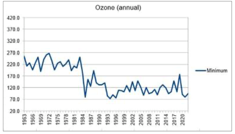
Remember when the UN Leftists had us ban all CFC’s to save the planet from Ozone depletion?
It did nothing other than add cost and regulation and gave a test run for banning CO2, Stoves, Meat and apparently fertilizer. Well they only want to ban the kind of fertilizer that works, as the fertilizer the EPA spills from it’s mouth is unlimited.
There are a lot of people who thing global warming is a hoax and others who think it is a real existential threat to society. Both are completely 100 percent wrong. Like most things, reality lies in the middle.
First, it is well known that there is no threat to existence from anthropogenic global warming. We know this from the body of work called ‘science’.
No trend in hurricanes No trend in drought No trend in rain No the fish are not shrinking No butterflies are going extinct Polar bears are doing great Antarctic ice is not shrinking away Sea level rise is a dead straight line for 150 years Penguins are doing great too.
That is all scientifically true. Yet how can some claim different? Well a lot of it is media exaggeration of single science papers which many of us consider outliers from the main body of work. However, there are a group of main-stream climate scientists who have learned to exaggerate and even lie about their work as it brings easy fame and fortune. Yes you communists, government money is fortune too and it corrupts just as well as the non-existent oil money would, were it actually being spent on science.
So what I want to write about are a few TRUE conspiracies to corrupt climate science and exaggerate risk. These are just examples but these are the real problems we should be discussing in the political world. Unfortunately, the indoctrinated cannot hear these words no matter how logical or documented they are.
Sea Level Rise
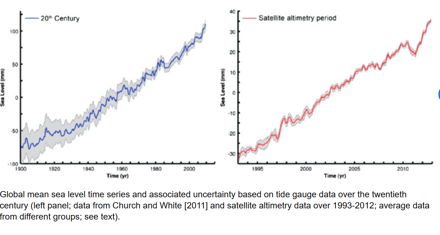
This is a very critical piece of climate change as the majority of atmospheric energy is held in the oceans. Warming would cause both melting and a physical expansion of the ocean water. Both would lead to sea level rise. Despite the fact that minimal warming has been detected with thousands of ground stations and somewhere around a dozen satellites, the ocean has not responded in any significant manner. It is literally rising at the same rate as it always has since before the invention of the internal combustion engine.
We have had zero measured impact on it – per the NOAA.
You can see on the left panel (tide gauge data for over a century) that there is no curvature to the graph since 1960 where global warming supposedly got serious. The panel on the right also has no visible curvature and it is from satellite data since 1993. So what would a conspiracy to make acceleration of sea level rise a real thing look like?
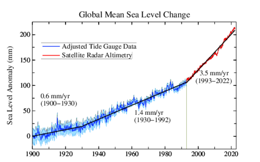
Well, paste em together and hide the recent dead-straight line of the tide gauge data (duh you dumas):
Instant curvature as provided by FAKE science from Columbia EDU. This is a conspiracy to convince morons that sea level rise is accelerating when clearly in the first graph, anyone can see that IT IS NOT CHANGING. This graph with fake curvature, makes the money. BTW, the little 1930 hitch is likely caused by the introduction of different tide gauge stations but it doesn’t matter to us as global warming didn’t start then.
Climate Models Fail Statistically
Climate models are used to determine the future state of climate. In the case of CO2, they are used to determine future temperatures based on different CO2 scenarios. These are similar to weather models except that they don’t work on micro scales and when the right parameters are given to them, like weather models, they can predict the future climate state based on whatever assumptions are given to them. Also, like weather models, their look-forward abilities are not perfect and they will diverge in time. Fortunately for climate scientists, when climate models are wrong, it takes decades to find out and the scientists can retire before their theories are proven inaccurate. For weather modelers, you know how well you did within days or weeks.
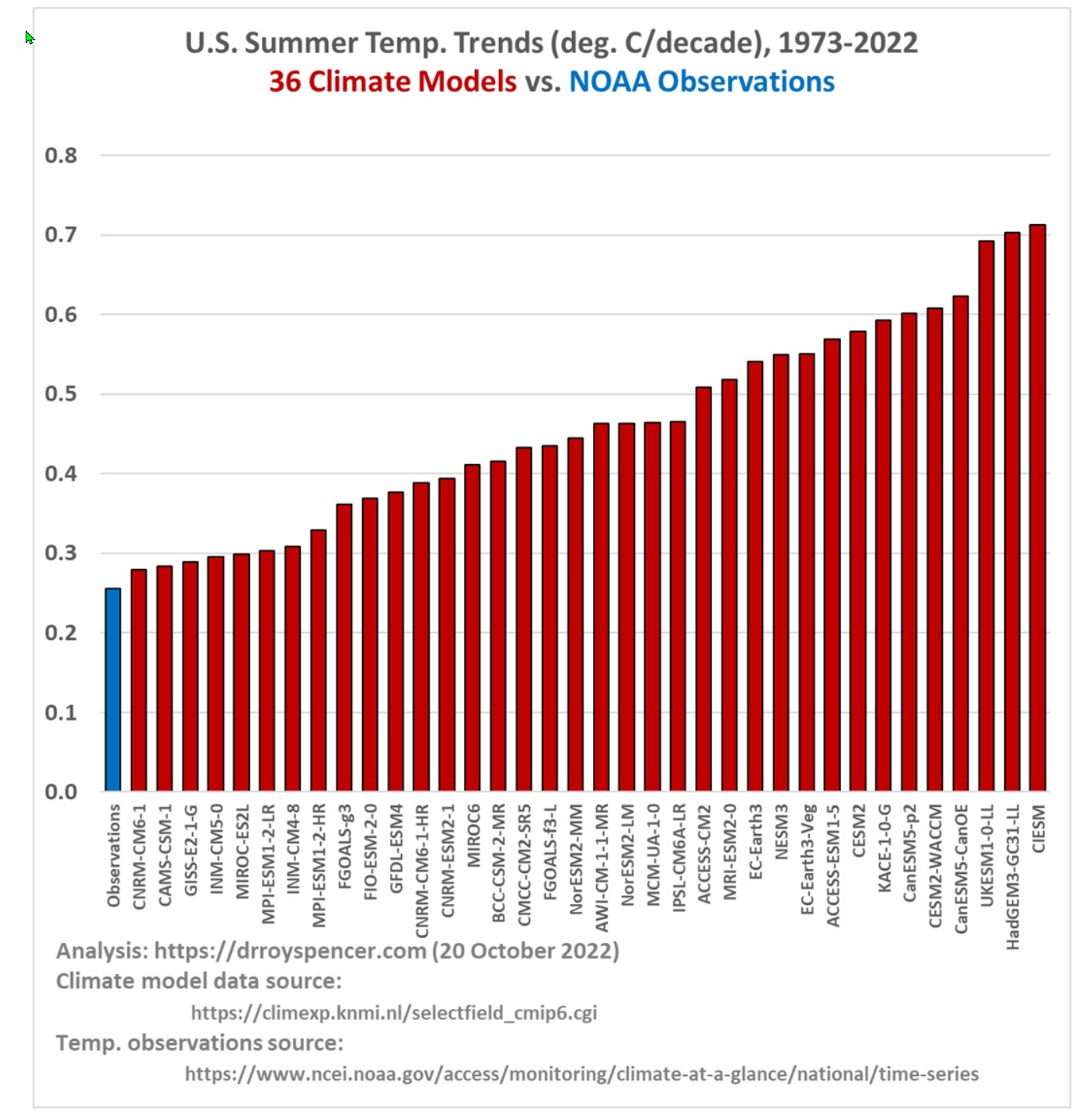
That whole lag in feedback leads to a commitment by climate modelers that they believe they are correct, followed by a feedback from actual weather decades later which unsurprisingly does not match. You can see on the far left side of the graph, NOAA measured temperatures — and on the right — every single climate model of note. DOH!!!
Why is this important, well because these models are expecting much warmer temperatures, even existential threat temperatures in the far future. Yet they over-predicted the observed warming in a much shorter timescale. If they are this wrong already, imagine how wrong they will be in 100 years. In other words, the planet temperature is NOT NEARLY AS SENSITIVE TO CO2 AS THEY CLAIM!!! All those models and not a single one got warming right on even a 30 year timescale. You would expect an unbiased attempt to have equal high and low misses. One hundred percent of the models over-predict warming.
And why is that important, well because by the numbers, this low of a temperature sensitivity to CO2 increases means we literally CANNOT destroy the planet by releasing CO2. The magnitude of the effect is not large enough, and the science is in. Don’t worry climate gaian’s, you cannot kill a multi-hundred billion dollar religion by simple facts. It takes a lot more than facts to shake the truth of the indoctrinated class. That climate science doesn’t address the problem is a conspiracy to hide the truth of the matter. Instead the science has worked hard to find corrections to observation to make them appear even slightly warmer. There even have been alarmist papers trying to obfuscate the problem, and the funny bit is, the papers wouldn’t exist if the problem they don’t want us to know about didn’t exist.
We believe in Truth over Facts
Joseph Biden – Subject words capitalized as that’s how he seems to mean them.
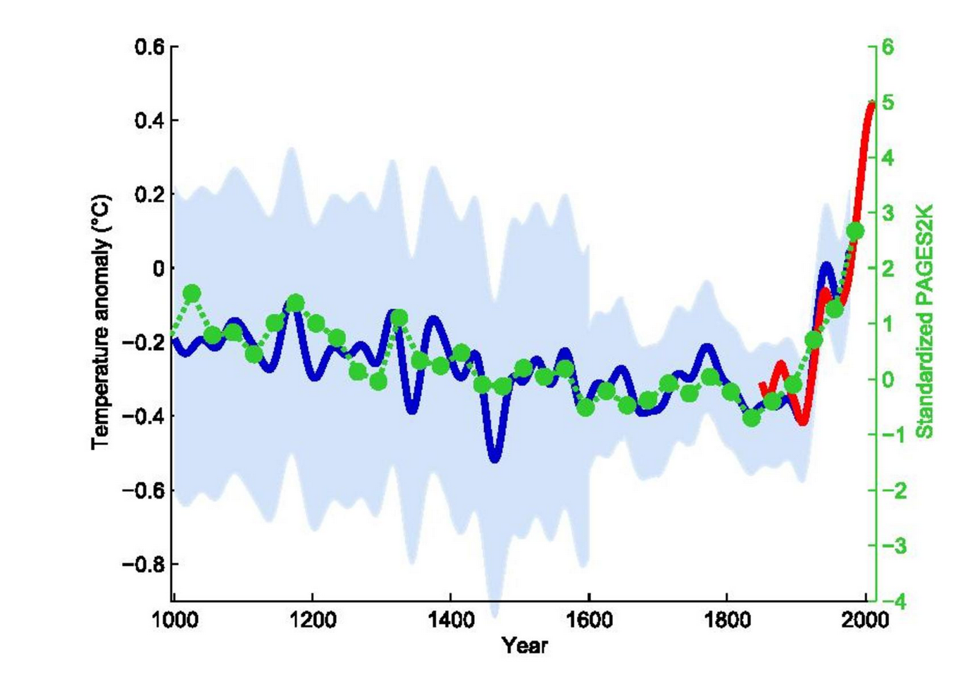
You can see temperatures in recent years are higher than any time in human history. Unfortunately for us all, this graph is completely bogus. It is FAKE beyond words. There is actually no data of use in it and no matter what data you feed the mathematical algorithm used to make this graph, you get the result you are looking for and a flat handle everywhere else. I’ve demonstrated the effect dozens of times using numerous methods. The simplest methods are shown here. In that post I use the same math and the same data as Mann08 used to show unprecedented temperatures to demonstrate all kinds of ridiculous results. While Mann appears to believe his own work, the rest of climate science has a serious problem with it. They still accept it though due to it’s unprecedented message. This is a conspiracy to convince you that global warming is serious and unprecedented and that we need to take socialism as the solution.
Some quotes from famous climatologists.
the results of this study will show that we can probably say a fair bit about <100 year extra-tropical NH temperature variability (at least as far as we believe the proxy estimates), but honestly know fuck-all about what the >100 year variability was like with any certainty (i.e. we know with certainty that we know fuck-all).
Ed Cook — Climategate Email Dump. This means that he believes that some of the tiny squiggles might be temperature, but the larger movements that don’t happen in the hockey stick handle are bogus. E.g. we don’t know that temperatures are unprecedented. I personally love this quote but challenge ed to show me why the short term squiggles are somehow temperature correlated — they are also just noise.
And another famous quote, also from climategate. The “scientists” are conspiring to delete data they don’t like and replace it with data they do like while not telling the reviewers. This is a common practice in the FAKE hockey stick world. Michael Mann just won a lawsuit for defamation because someone said he was a fraud. I have never made that claim but now we know with certainty, due to the brilliance of a DC jury, that he is not a fraud.
I’ve just completed Mike’s Nature trick of adding in the real temps to each series for the last 20 years (ie from 1981 onwards) amd [sic] from1961 for Keith’s to hide the decline.
Phil Jones – Climategate Email Dump
Literally deleting data by hand that doesn’t match the narrative, as apparently had been done before in the journal Nature.
Because of the evidence for loss of temperature sensitivity after 1960 (1), MXD data were eliminated for the post-1960 interval.
Mann 08, an actual hockeystick paper
From: Mick Kelly Subject: RE: Global temperature Date: Sun, 26 Oct 2008 09:02:00 +1300
Yeah, it wasn’t so much 1998 and all that that I was concerned about, used to dealing with that,but the possibility that we might be going through a longer – 10 year – period of relatively stable temperatures beyond what you might expect from La Nina etc. Speculation, but if I see this as a possibility then others might also. Anyway, I’ll maybe cut the last few points off the filtered curve before I give the talk again as that’s trending down as a result of the end effects and the recent cold-ish years.
Enjoy Iceland and pass on my best wishes to Astrid.
Mick
Climategate Email Dump
So there you have it, another exposed climate conspiracy. So this is what climate science boils down to:
CO2 warming is real, it is small and it is not at all dangerous, in fact it seems wildly beneficial in that plant-life (actual planetary greening) is blooming like never before. Global warming insanity however, has reached the level of a religion that cannot be opposed. It is funded by hundreds of billions of dollars per year through layers and layers of hidden networks. I’ve spent many hours trying to figure out which money went where. Good luck with that job friends.
Anyway, there are numerous other aspects of this science that are exaggerated and even totally fake. For instance, the Antarctic will not be melting any time in the next 5 millennia – because it is way too cold. Those that tell you otherwise, are simply charlatans.
So the science is sometimes, but not always, exaggerated the UN IPCC exaggerates the conclusions further, and the media takes it to the wall. EXISTENTIAL THREAT!!!! Politicians use the fear to take your freedom and money.
Cars, stoves, refrigerators, air-conditioning, heating, energy generation, foods, land and even fertilizer. There is no end to the limitations they will impose on you, all for an exaggerated science that is full of conspiracy.
So it seems that one of the main methods used in Democrat vote fraud was ballot return from bad addresses. Somehow, undeliverable ballots were collected, filled out and returned fraudulently. It seems irrational to think that the post offices had wide-spread involvement in such a scheme but here is a set of videos including a postal worker placing dozens of ballots in drop boxes on multiple trips.
So people love to say that this is not proof. Today Gateway Pundit has an important article about a lady who “tested the system” by using registered military members identification to send absentee ballots to unaffiliated addresses. She got prosecuted and found guilty. It appears that there were only 3 ballots identified but I don’t have the court transcripts.
However, check out this little nugget by The Gateway Pundit.
The Gateway Pundit has reported extensively on this 2020 voter fraud scheme in several battleground states where military ballots shockingly went almost entirely to Joe Biden. We posted evidence that this occurred in Michigan, Arizona and Georgia.
The same method worked in Wisconsin.
We need to have, in person, citizen only, photo voter identification.
You will be required to buy non-functional and extremely expensive transportation. This transportation will drive costs through the roof, eliminate development on more efficient internal combustion, damage the oil and gas industries, overload the ZERO-PLANNING electric generation industry and crash the economy — unsurprisingly leading to government dependence.
All in the name of the extraordinarily exaggerated and unscientifically invented problem of CO2, which EV’s do little to address.
Even if we magically stop this law, unless we stop the unconstitutional law making by unelected federal agencies, the US is lost. And so is the rest of the world.
Alliance for Automotive Innovation President and CEO John Bozzella noted Wednesday that, while the EPA’s adjusted EV targets are “still a stretch goal,” they were more reasonable than the ones first proposed.
“Moderating the pace of EV adoption in 2027, 2028, 2029 and 2030 was the right call because it prioritizes more reasonable electrification targets in the next few years of the EV transition,” he said.
Fox News
I just have to add, that the government does not decide what we buy. That is not their role and for an unelected agency, that happens to be 95 plus percent pro-government communist controlled in Washington DC to think that this is their role in life, is disgusting beyond words. America is a free capitalist country and should remain so as that is what gave us our success.
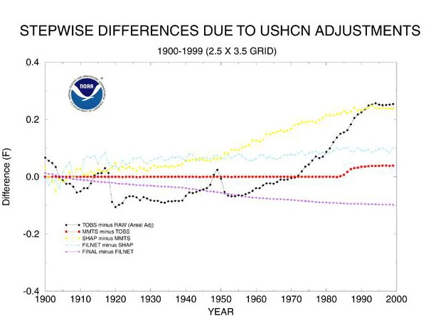
Just to make the point about US temperature corrections, below is a plot of how the US temperature record is adjusted from raw data. The raw data actually has very little trend, however there are problems in the collection method of this data that require significant adjustments for accuracy.
Figure 2. Form of individual corrections applied by NOAA. The black line is the adjustment for time of observation. The red line is for a change in maximum/minimum thermometers used. The yellow line is for changes in station siting. The pale blue line is for filling in missing data from individual station records. The purple line is for UHI effects (this correction is now removed).
Jennifer Marohasy blog.
And so there you have it. The vast conspiracy theorists are correct. About half of the US temperature increase is due to adjustments in the record. These adjustment are correct and necessary as far as I can tell.
Just thought I would add the link to an article which I also had written a year ago. People need to understand that all that big mean global warming heat has to be going somewhere and the water is the only place in our climate system — if the heat energy is real. There must be an increase in the rate of sea level rise or we all have to agree that CO2 warming is very small.